By Bob Rudis (@hrbrmstr)
Fri 13 June 2014 | tags: rstats, r, datavis, wifi, cartography, maps, RCurl, -- (permalink)

This is the second of a two-part series. Part 1 set up the story and goes into how to discover, digest & reformat the necessary data. This concluding segment will show how to perform some basic visualizations and then how to build beautiful & informative density maps from the data and offer some suggestions as to how to prevent potential tracking.

I’ll start with the disclaimer from the previous article:

DISCLAIMER I have no proof—nor am I suggesting—that Xfinity or BSG Wireless is actually maintaining records of associations or probes from mobile devices. However, the ToS & privacy pages on each of their sites did not leave me with any tpye of warm/fuzzy feeling that this data is not—in fact—being used for tracking purposes.

Purely by coincidence, @NPRNews‘ Steve Henn also decided to poke at Wi-Fi networks during their cyber series this week and noted other potential insecurities of Comcast’s hotspot network. That means along with tracking, you could also be leaking a great deal of information as you go from node to node. Let’s see just how pervasive these nodes are.

Visualizing Hotspots

Now, you don’t need the smartphone app to see the hotspots. Xfinity has a web-based hotspot finder based on Google Maps:

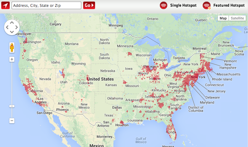
Those “dots” are actually bitmap tiles (even as you zoom in). Xfinity either did that to “protect” the data, save bandwidth or speed up load-time (creating 260K+ points can take a few, noticeable seconds). We can reproduce this in R without (and with) Google Maps pretty easily:

library(maptools)
library(maps)
library(rgeos)
library(ggcounty)

# you can grab ggcounty via:
# install.packages("devtools")
# install_github("hrbrmstr/ggcounty")

# grab the US map with counties

us <- ggcounty.us(color="#777777", size=0.125)

# plot the points in "Xfinity red" with a 
# reasonable alpha setting & point size

gg <- us$gg
gg <- gg %+% xfin + aes(x=longitude, y=latitude)
gg <- gg + geom_point(color="#c90318", size=1, alpha=1/20)
gg <- gg + coord_map(projection="mercator")
gg <- gg + xlim(range(us$map$long))
gg <- gg + ylim(range(us$map$lat))
gg <- gg + labs(x="", y="")
gg <- gg + theme_bw()

# the map tends to stand out beter on a non-white background
# but the panel background color isn't truly "necessary"

gg <- gg + theme(panel.background=element_rect(fill="#878787"))
gg <- gg + theme(panel.grid=element_blank())
gg <- gg + theme(panel.border=element_blank())
gg <- gg + theme(axis.ticks.x=element_blank())
gg <- gg + theme(axis.ticks.y=element_blank())
gg <- gg + theme(axis.text.x=element_blank())
gg <- gg + theme(axis.text.y=element_blank())
gg <- gg + theme(legend.position="none")
gg

library(ggmap)

x_map <- get_map(location = 'united states', zoom = 4, maptype="terrain", source = 'google')
xmap_gg <- ggmap(x_map)

gg <- xmap_gg %+% xfin + aes(x=longitude, y=latitude)
gg <- gg %+% xfin + aes(x=longitude, y=latitude)
gg <- gg + geom_point(color="#c90318", size=1.5, alpha=1/50)
gg <- gg + coord_map(projection="mercator")
gg <- gg + xlim(range(us$map$long))
gg <- gg + ylim(range(us$map$lat))
gg <- gg + labs(x="", y="")
gg <- gg + theme_bw()
gg <- gg + theme(panel.grid=element_blank())
gg <- gg + theme(panel.border=element_blank())
gg <- gg + theme(axis.ticks.x=element_blank())
gg <- gg + theme(axis.ticks.y=element_blank())
gg <- gg + theme(axis.text.x=element_blank())
gg <- gg + theme(axis.text.y=element_blank())
gg <- gg + theme(legend.position="none")
gg

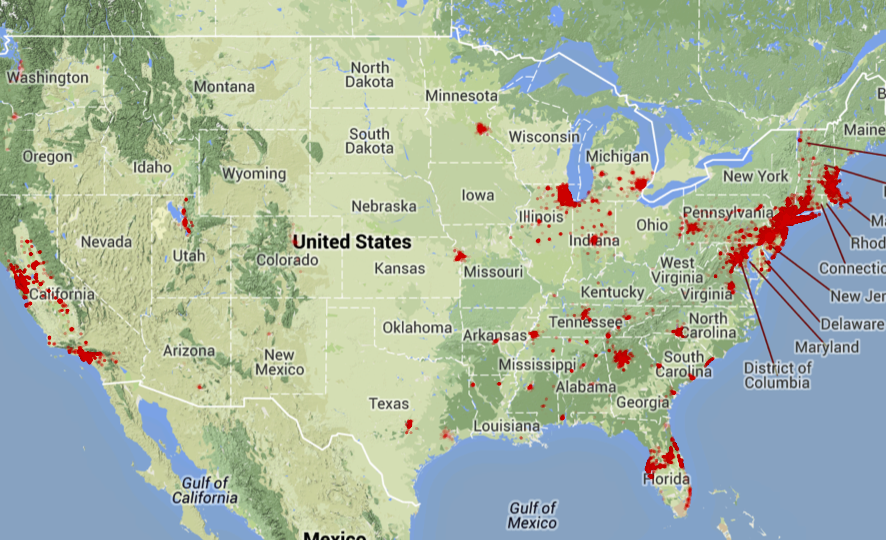
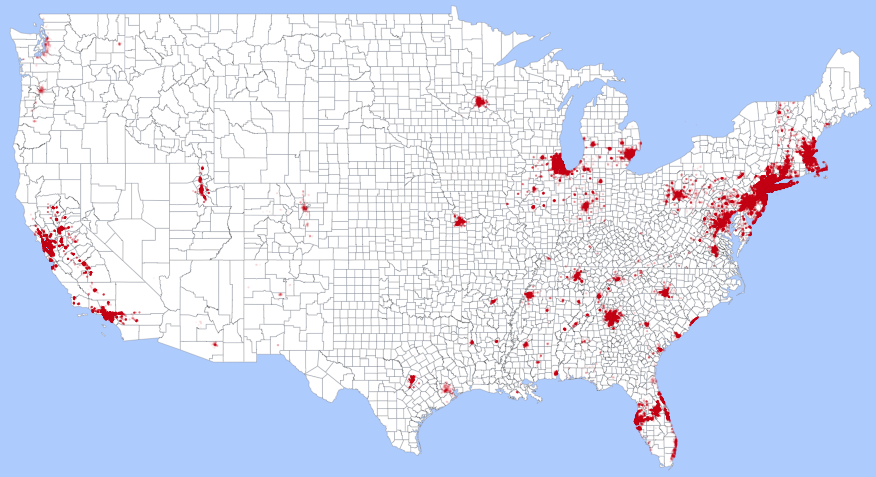
It’s a bit interesting that they claim over a million hotspots but the database has less then 300K entries.

I made the dots a bit smaller and used a fairly reasonable alpha setting for them. However, the macro- (i.e. the view of the whole U.S.) plus dot-view really doesn’t give a good feel for the true scope of the coverage (or possible tracking). For that, we can turn to state-based density maps.

There are many ways to generate/display density maps. Since we’ll still want to display the individual hotspot points as well as get a feel for the area, we’ll use one that outlines and gradient fills in the regions, then plot the individual points on top of them.

library(ggcounty)

l_ply(grep("Idaho", unique(xfin$county), value=TRUE, invert=TRUE), function(state) {

  print(state) # lets us know progress as this takes a few seconds/state

  gg.c <- ggcounty(state, color="#737373", fill="#f0f0f0", size=0.175)

  gg <- gg.c$gg
  gg <- gg %+% xfin[xfin$county==state,] + aes(x=longitude, y=latitude)
  gg <- gg + stat_density2d(aes(fill=..level.., alpha=..level..), 
                            size=0.01, bins=100, geom='polygon')
  gg <- gg + scale_fill_gradient(low="#fddbc7", high="#67001f")
  gg <- gg + scale_alpha_continuous(limits=c(100), 
                                    breaks=seq(0, 100, by=1.0), guide=FALSE)
  gg <- gg + geom_density2d(color="#d6604d", size=0.2, alpha=0.5, bins=100)
  gg <- gg + geom_point(color="#1a1a1a", size=0.5, alpha=1/30)
  gg <- gg + coord_map(projection="mercator")
  gg <- gg + xlim(range(gg.c$map$long))
  gg <- gg + ylim(range(gg.c$map$lat))
  gg <- gg + labs(x="", y="")
  gg <- gg + theme_bw()
  gg <- gg + theme(panel.grid=element_blank())
  gg <- gg + theme(panel.border=element_blank())
  gg <- gg + theme(axis.ticks.x=element_blank())
  gg <- gg + theme(axis.ticks.y=element_blank())
  gg <- gg + theme(axis.text.x=element_blank())
  gg <- gg + theme(axis.text.y=element_blank())
  gg <- gg + theme(legend.position="none")

  ggsave(sprintf("output/%s.svg", gsub(" ", "", state)), gg, width=8, height=8, units="in", dpi=140)
  ggsave(sprintf("output/%s.png", gsub(" ", "", state)), gg, width=6, height=6, units="in", dpi=140)

})

The preceeding code will produce a density map per state. Below is an abbreviated gallery of (IMO) the most interesting states. You can click on each for a larger (SVG) version.

Some of SVGs have a hefty file size, so they might take a few seconds to load.

You can also single out your own state for examination:

Now, these are just basic density maps. They don’t take into account Wi-Fi range, so the areas are larger than actual signal coverage. The purpose was to show just how widespread (or minimal) the coverage is vs convey discrete tracking precision. As you jump from association to association, it would be trivial for any provider to “connect the dots”.

Covering Your Tracks

Comcast (Xfinity) and AT&T aren’t the only places where this tracking can occur. CreepyDOL was demoed at BlackHat in 2013 (making it pretty simple for almost anyone to setup tracking). Stores already use your Wi-Fi associations to track you. Navizon has a whole product/service based on the concept.

Apple is trying to help with a new feature in iOS 8 that will randomize MAC addresses when probing for access points and David Schuetz has advocated deleting preferred networks from your iOS networks list.

What can you do while you wait for iOS (and wait even longer for the framented Android world to catch up)? Android users can give AVG’s new PrivacyFix a go, but one of your only direct controls is to disable Wi-Fi, but that might not truly help if your mobile operating system does not deal well with passive Wi-Fi probes. Another option (as mentioned above) is to regularly purge the list of previously associated networks. You could even go so far as to bundle up your phone and stop all signales coming in and out, but that somewhat defeats the purpose of having your mobile with you.

Remain aware that the tracking can happen invisibly anywhere and, perhaps more importantly, the dangers that open Wi-Fi networks pose in general. Use a VPN service like Cloak to at least ensure all your transmissions are free from local prying eyes so the trackers have as little data to associate with you as possible.

Finally, keep putting pressure on the FTC to help with this privacy issue. While FTC/FCC efforts won’t stop malicious actors, it might help reign in businesses and encourage more privacy innovation on the part of Apple/Android/Microsoft.