
By Bob Rudis (@hrbrmstr)
Fri 02 January 2015
|
tags:
blog,
rstats,
r,
ipv4,
ip address,
hilbert,
-- (permalink)
While there’s an unholy affinity in the infosec commuinty with slapping IPv4 addresses onto a world map, that isn’t the only way to spatially visualize IP addresses. A better approach (when tabluation with bar charts, tables or other standard visualization techniques won’t do) is to map IPv4 addresses into Hilbert space-filling curve. You can get a good feel for how these work over at The Measurement Factory, which is where this image comes from:

This paper [PDF] also is a good primer.
While TMF’s ipv4heatmap command-line software can crank out those visualizations really well, I wanted a way to generate them in R as we explore internet IP space at work. So, I adapted bits of their code to work in a ggplot context and took a stab at an ipv4heatmap package.
The functionality is currently pretty basic. Give ipv4heatmap a vector of IP addresses and you’ll get a heatmap of them. Feed in a CIDR block to boundingBoxFromCIDR and you’ll get a structure suitable for displaying with geom_rect. To get an idea of how it works, here’s a small example.
The following snippet of code reads in a cached copy of an IPv4 block list from blocklist.de and turns the IP addresses into a heatmap (which is mostly one color since there aren’t many blocks per class C). It then grabs the CIDR blocks for China and North Korea since, well, #CHINADPRKHACKSALLTHETHINGS according to “leading” IR firms and the US gov. It then overlays a alpha filled rectangle over the map to see just how many points fall within those CIDRs.
devtools::install_github("vz-risk/ipv4heatmap")
library(ipv4heatmap)
library(data.table)

# read in cached copy of blocklist.de IPs - orig URL https://www.blocklist.de/en/export.html
hm <- ipv4heatmap(readLines("https://datadrivensecurity.info/data/all.txt"))

# read in CIDRs for China and North Korea
cn <- read.table("https://www.iwik.org/ipcountry/CN.cidr", skip=1)
kp <- read.table("https://www.iwik.org/ipcountry/KP.cidr", skip=1)

# make bounding boxes for the CIDRs

cn_boxes <- rbindlist(lapply(boundingBoxFromCIDR(cn$V1), data.frame))
kp_box <- data.frame(boundingBoxFromCIDR(kp$V1))

# overlay the bounding boxes for China onto the IPv4 addresses we read in and Hilbertized

gg <- hm$gg
gg <- gg + geom_rect(data=cn_boxes,
                     aes(xmin=xmin, ymin=ymin, xmax=xmax, ymax=ymax),
                     fill="white", alpha=0.2)
gg <- gg + geom_rect(data=kp_box,
                     aes(xmin=xmin, ymin=ymin, xmax=xmax, ymax=ymax),
                     fill="white", alpha=0.2)

gg
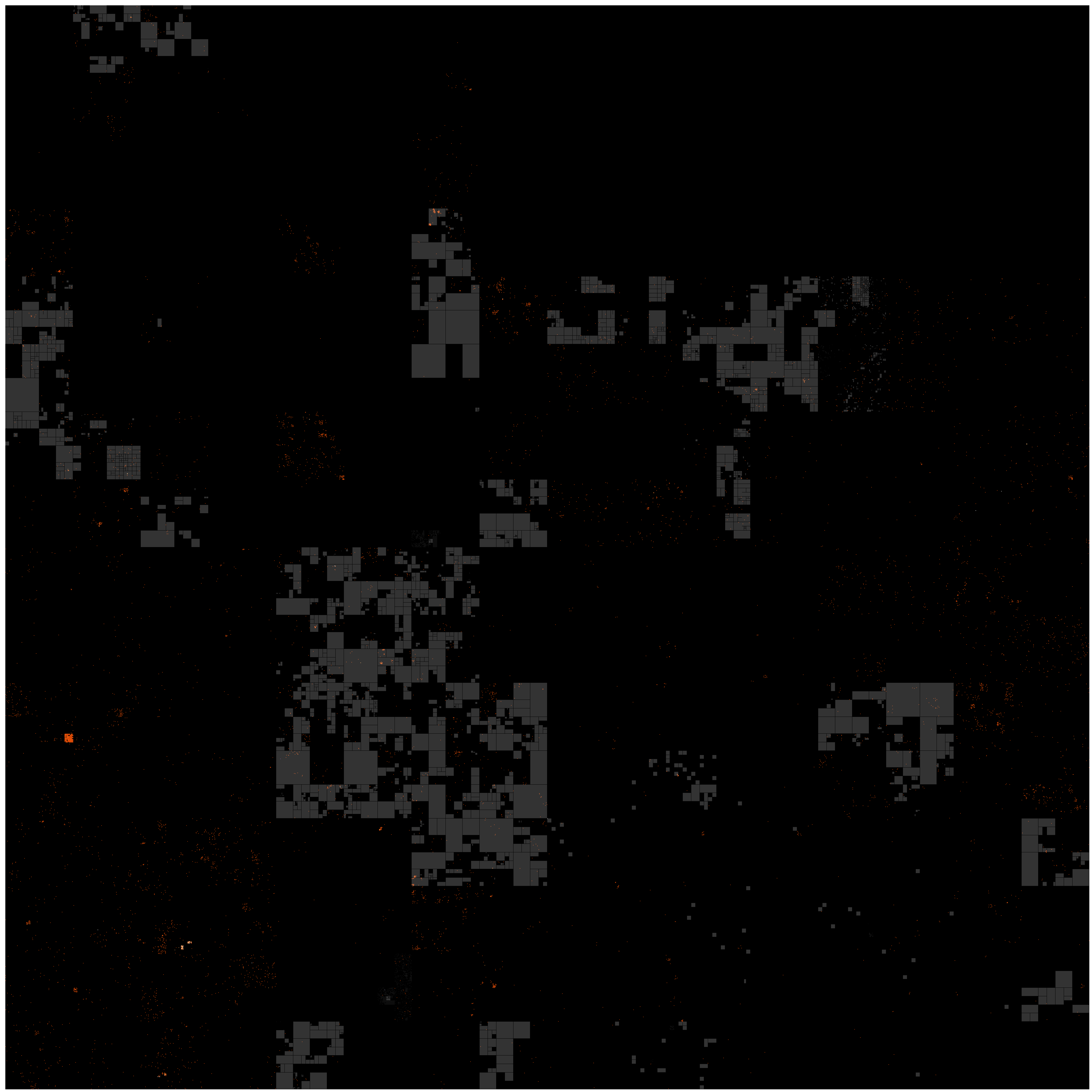
You’ll want to download that and open it up in a decent image program. The whole image is 4096x4096, so you can zoom in pretty well to see where evil hides itself.
If you find a cool use for ipv4heatmap definitely drop a note in the comments or on github. One thing we’ve noticed is that wrapping a series of individual images up in animation to see changes over time can be really interesting/illuminating.
One caveat: it uses the Boost libraries, so Windows R folk may need to jump through some hoops to get it going.
Countries Of The Internet
Since I was playing around with IPv4 heatmaps, I thought it might be neat to show how country IP address allocations fit on the “map”. So, I took the top 12 countries (by # of IPv4 addresses assigned), used ipv4heatmap to color in their bounding boxes and then whipped up some javascript to let you see/explore the fragmented allocation landscape we live in.
There’s also a non-framed version of that available. The 2D canvas scaling may be off in some browsers, but not by much. Shift-click once in the image to compensate if it’s cut off at all.
The amount of “micro-allocation” (my term) really surprised me. While I “knew” it was this way, seeing it gives you a whole new perspective.
The more I’ve worked with routing, IP & DNS data over the years, the more I’m amazed that anything on the internet works at all.
Tweet