
By Bob Rudis (@hrbrmstr)
Sat 18 January 2014
|
tags:
shiny,
R,
-- (permalink)
An innocent thread on the SIRA mailing list begat a detailed explanation by Jay which begat a comment with a link to a gist by David Severski that had an equally innocent comment:
# extending to UI framework of your choice is left as an exercise for the reader
(see Jay’s post & David’s gist for complete context)
In a nutshell, David made a great R simulation of a FAIR risk analysis. So great, in fact, that it was really straightforward to turn it into a Shiny app. To quote from their site: “Shiny makes it super simple for R users like you to turn analyses into interactive web applications that anyone can use.”
Readers will no doubt be seeing many Shiny apps from DDS over the coming months/years. I will refrain from duplicating content in the extremely helpful Shiny tutorial series, so you should head over there and read through that first before continuing here.
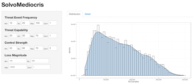
In their most basic form, Shiny apps are defined by a user interface component : ui.R : and a back-end processing component : server.R (once you dig into Shiny, you’ll see what a gross over-simplification that truly is). David’s code was in almost perfect form for the server-component, and it was relatively straightforward to make a basic user-interface for it. But, a picture is worth a thousand words: (you can click on the image to go right to the DDS SolvoMediocris Shiny app).
The interface is extremely dynamic (i.e. whenever any value changes, the risk simulation is re-run). Extending it to add a button for running the simulation is an exercise left for the reader (I hacked this out really quickly).
Here’s the ui.R code:
shinyUI(pageWithSidebar(

    headerPanel("SolvoMediocris"),

    sidebarPanel(

            tags$head(
        tags$style(type="text/css", "input { font-size:10px; width:40px; display:inline-block; }"),
        tags$style(type="text/css", "#lml, #lmml, #lmh, #lmconf { font-size:10px; width:100px; display:inline-block; }"),
        tags$style(type="text/css", "label { font-size:10px; display:inline-block; }")
            ),

            h4("Threat Event Frequency"),
        numericInput("tefl", "Min:", 10, min = 0, max = 100),
        numericInput("tefml", "ML:", 20, min = 0, max = 100),
        numericInput("tefh", "Max:", 100, min = 0, max = 100),
        numericInput("tefconf", "Conf:", 1, min = 1, max = 5),

            h4("Threat Capability"),
        numericInput("tcapl", "Min:", 20, min = 0, max = 100),
        numericInput("tcapml", "ML:", 30, min = 0, max = 100),
        numericInput("tcaph", "Max:", 70, min = 0, max = 100),
        numericInput("tcapconf", "Conf:", 1, min = 1, max = 5),

            h4("Control Strength"),
        numericInput("csl", "Min:", 40, min = 0, max = 100),
        numericInput("csml", "ML:", 50, min = 0, max = 100),
        numericInput("csh", "Max:", 60, min = 0, max = 100),
        numericInput("csconf", "Conf:", 2, min = 1, max = 5),

            h4("Loss Magnitude"),
        numericInput("lml", "Min:", 100, min = 0),
        numericInput("lmml", "ML:", 500, min = 0), br(),
        numericInput("lmh", "Max:", 10000, min = 0),
        numericInput("lmconf", "Conf:", 1, min = 1, max = 5), br(),

            div(HTML("<small>(App brought to you by <a href='https://datadrivensecurity.info'>Data Driven Security</a>)</small>"))

    ),

    mainPanel(
        tabsetPanel(
            tabPanel("Distribution", plotOutput("plot")),
            tabPanel("Detail", verbatimTextOutput("detail"), verbatimTextOutput("detail2"))
        )
    )

))
As you can see, (hopefully) it’s pretty readable/digestible without much explanation. Shiny lets you use templates and you can even use raw HTML with callbacks to the server. However, as you can see it’s quick work to use the “HTML functions” exposed by the shiny package to knock out a basic interface. The tef…, tcap… etc names become input$tef… variables on the server and the innate “reactive” functionality of the Shiny framework makes it super-simple to process those values as they change. The mainPanel() function defines the output areas for what the server will generate.
The server side is pretty lean as you can see in server.R:
library(shiny)
library(mc2d)
library(ggplot2)
library(scales)

N <- 50000

shinyServer(function(input,output){

        simulate <- reactive( {

            TEFestimate <- data.frame(L = input$tefl,  ML = input$tefml,  H = input$tefh, CONF = input$tefconf)
            TSestimate <- data.frame(L = input$tcapl,  ML = input$tcapml,  H = input$tcaph, CONF = input$tcapconf)
            RSestimate <- data.frame(L = input$csl,  ML = input$csml,  H = input$csh, CONF = input$csconf)
            LMestimate <- data.frame(L = input$lml, ML = input$lmml, H = input$lmh, CONF = 1)

            LMsample <- function(x){
              return(sum(rpert(x, LMestimate$L, LMestimate$ML, LMestimate$H, shape = LMestimate$CONF) ))
            }

            TEFsamples <- rpert(N, TEFestimate$L, TEFestimate$ML, TEFestimate$H, shape = TEFestimate$CONF)
            TSsamples <- rpert(N, TSestimate$L, TSestimate$ML, TSestimate$H, shape = TSestimate$CONF)
            RSsamples <- rpert(N, RSestimate$L, RSestimate$ML, RSestimate$H, shape = RSestimate$CONF)

            VULNsamples <- TSsamples > RSsamples
            LEF <- TEFsamples[VULNsamples]

            return(sapply(LEF, LMsample))

        })

    output$plot <- renderPlot({

            ALEsamples <- simulate()

            gg <- ggplot(data.frame(ALEsamples), aes(x = ALEsamples))
            gg <- gg + geom_histogram(binwidth = diff(range(ALEsamples)/50), aes(y = ..density..), color = "black", fill = "white")
            gg <- gg + geom_density(fill = "steelblue", alpha = 1/3)
            gg <- gg + scale_x_continuous(labels = comma)
            gg <- gg + theme_bw()

            print(gg)

    })

    output$detail <- renderPrint({
            ALEsamples <- simulate()
            print(summary(ALEsamples));
    })

    output$detail2 <- renderPrint({
            ALEsamples <- simulate()
            VAR <- quantile(ALEsamples, probs=(0.95))
            print(paste0("Losses at 95th percentile are $", format(VAR, nsmall = 2, big.mark = ",")));
    })

})
Anytime one of the input variables changes, simulate “invalidates” and the simulation is re-run and the outputs (plot and data)are updated.
We’ll cover Shiny in more detail in upcoming posts and as we build more apps. In the meantime, you can grab these source files over at our gist, play with the app and drop a note in the comments if you have any questions.
Tweet