By Bob Rudis (@hrbrmstr)
Fri 29 August 2014
|
tags:
dns,
tlds,
dplyr,
r,
rstats,
-- (permalink)
I saw this on Hacker News this morning and it got me curious as to how many other TLDs (e.g. .com) resolve to an address (i.e. https://uz./ displays a page in your browser since uz. resolves to 91.212.89.8). This is quick work with R and the resolv & iptools packages, plus I threw in a little dplyr for good measure:
library(iptools)
library(resolv)
library(dplyr)
library(ggplot2)

data(ianarootzonetlds) # iptools has IANA TLDs data built in

# iterate over the TLDs; try an A lookup getting NA back if bad
# could have used A() but originally intended to do more with the data

whichresolve <- sapply(ianarootzonetlds$Domain, function(x) {
  y <- resolv_a(sprintf("%s.", gsub(".", "", x, fixed=TRUE)))
  if (length(y) > 0) { y } else { NA }
})

tlds <- data.frame(ianarootzonetlds$Domain, whichresolve)
rownames(tlds) <- NULL

# which ones weren't NA == they have an IP address
# dplyr lets us use "pipes" (similar to unix pipes)
# to pass data around and it's far more readable than
# sticking conditionals in tons of nested brackets

tlds %>% filter(!is.na(whichresolve))

##    ianarootzonetlds.Domain   whichresolve
## 1                      .ac 193.223.78.210
## 2                  .active    127.0.53.53
## 3                      .ai  209.59.119.34
## 4                   .autos    127.0.53.53
## 5                     .bmw    127.0.53.53
## 6                      .cm  195.24.205.60
## 7                      .dk 193.163.102.24
## 8                      .gg  87.117.196.80
## 9                   .green    127.0.53.53
## 10                  .homes    127.0.53.53
## 11                     .io 193.223.78.212
## 12                     .je  87.117.196.80
## 13                   .lgbt    127.0.53.53
## 14                  .lotto    127.0.53.53
## 15                   .meet    127.0.53.53
## 16                   .mini    127.0.53.53
## 17            .motorcycles    127.0.53.53
## 18                    .ngo    127.0.53.53
## 19                    .nra    127.0.53.53
## 20                     .pn   80.68.93.100
## 21                     .sh 193.223.78.211
## 22                .spiegel    127.0.53.53
## 23                     .tk  217.119.57.22
## 24                     .tm 193.223.78.213
## 25                     .to  216.74.32.107
## 26                     .uz    91.212.89.8
## 27                     .ws    64.70.19.33
## 28                 .yachts    127.0.53.53

# since we can eyeball one very common IP address, see how common it is
# and use a fairly common dplyr chain to get the results

tlds %>%
  filter(!is.na(whichresolve)) %>% # exclude some
  group_by(whichresolve) %>%       # group by IP
  tally() %>%                      # get a count
  select(IP=whichresolve, n) %>%   # rename & select columns
  arrange(desc(n))                      # sort

##                IP  n
## 1     127.0.53.53 14
## 2   87.117.196.80  2
## 3  193.163.102.24  1
## 4  193.223.78.210  1
## 5  193.223.78.211  1
## 6  193.223.78.212  1
## 7  193.223.78.213  1
## 8   195.24.205.60  1
## 9   209.59.119.34  1
## 10  216.74.32.107  1
## 11  217.119.57.22  1
## 12    64.70.19.33  1
## 13   80.68.93.100  1
## 14    91.212.89.8  1
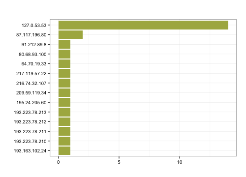
and use the dplyr chain directly with ggplot2 (and using Pantone’s “color of the day” for August 29th, 2014 for fun):
tlds %>%
  filter(!is.na(whichresolve)) %>%
  group_by(whichresolve) %>%
  tally() %>%
  select(IP=whichresolve, n) %>%    # magrittr/dplyr pipe works nicely with ggplot
  ggplot(aes(x=reorder(IP, n), y=n)) +
    geom_bar(stat="identity", fill="#ACB350") +
    coord_flip() + labs(x="", y="", title="") + theme_bw()

Out of 679 entries in the IANA TLDs, 28 resolve and, of those, 14 to the same IP address, which just happens to be the new “Name Collission” IP address. Excluding that address, there are just 13 unique IP addresses and only 14 domains that have an actual IPv4 address. For fun, we can see where those IPs “live”:
# using tbl_df() to make the output more compact
# feeding a "dplyr chained" column right into iptools' geoip()
# which is probably making Jay cringe right about now

tbl_df(geoip((tlds %>%
  filter(!is.na(whichresolve) & whichresolve != "127.0.53.53") %>%
  select(IP=whichresolve))$IP))

## Source: local data frame [14 x 13]
##
##                ip country.code country.code3   country.name region region.name         city
## 1  193.223.78.210           GB           GBR United Kingdom     NA          NA           NA
## 2   209.59.119.34           AI           AIA       Anguilla     00          NA   The Valley
## 3   195.24.205.60           CM           CMR       Cameroon     NA          NA           NA
## 4  193.163.102.24           DK           DNK        Denmark     NA          NA           NA
## 5   87.117.196.80           GB           GBR United Kingdom     NA          NA           NA
## 6  193.223.78.212           GB           GBR United Kingdom     NA          NA           NA
## 7   87.117.196.80           GB           GBR United Kingdom     NA          NA           NA
## 8    80.68.93.100           GB           GBR United Kingdom     NA          NA           NA
## 9  193.223.78.211           GB           GBR United Kingdom     NA          NA           NA
## 10  217.119.57.22           DE           DEU        Germany     NA          NA           NA
## 11 193.223.78.213           GB           GBR United Kingdom     NA          NA           NA
## 12  216.74.32.107           US           USA  United States     CA  California     Richmond
## 13    91.212.89.8           UZ           UZB     Uzbekistan     NA          NA           NA
## 14    64.70.19.33           US           USA  United States     MO    Missouri Chesterfield
## Variables not shown: postal.code (fctr), latitude (dbl), longitude (dbl), time.zone (fctr),
##   metro.code (int), area.code (int)
While the post did want to answer a certain question, one of the main goals was to give a sneaky introduction to working with dplyr. It’s a powerful new idiom in R that helps make code more logical, readable and (in most cases) much faster. A good place to learn more is over at the official introduction vignette.
