By Bob Rudis (@hrbrmstr)
Thu 18 September 2014
|
tags:
r,
rstats,
torrentfreak,
bittorrent,
pirate,
tlapd,
movies,
-- (permalink)

We leave the Jolly Roger behind this year and turn our piRate spyglass towards the digital seas and take a look at piRated movies as seen through the lens of TorrentFreak. The seasoned seadogs who pilot that ship have been doing a weekly “Top 10 Pirated Movies of the Week” post since early 2013, and I thought it might be fun to gather, process, analyze and visualize the data for this year’s annual TLAPD post. So, let’s weigh anchor and set sail!
NOTE: I’m leaving out some cruft from this post - such as all the
library()calls - and making use of comments in code snippets to help streamline the already quite long presentation. You can grab all the code+data over at it’s github repo. It will be much easier to run the R project code from there.
Since this is a code-heavy post, you’ve got the option to toggle the code segments for readability. Remember, too, that all lightbox-displayed images can be right-clicked/saved-as (or open tabbed) for full scale viewing.
PlundeRing the PiRate Data
To do any kind of analysis & visualization you need data (#CaptainObvious). While TorrentFreak has an RSS feed for their “top 10”, I haven’t been a subscriber to it, so needed to do some piRating of my own to get some data to work with. After inspecting their top 10 posts, I discovered that they used plain ol’ HTML <table>‘s for markup (which, thankfully, was very uniformly applied across the posts).
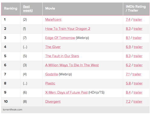
R excels at scraping data from the web, and I was able to use the new rvest package to grab the pages and extract the table contents. The function below iterates over every week since March 3, 2013, grabs the table from the page and stores it in a data frame. Note that there are two different formats for the URLs (I suspect that indicates multiple authors with their own personal standards for article slugs) that need to be handled by the function:
scrapeMovieData <- function() {

  # get all the Mondays (which is when torrentfreak does their top 10 post)
  # they seem to have started on March 3rd and the URL format varies slightly

  dates <- seq.Date(as.Date("2013-03-03"), as.Date("2014-09-17"), by="1 day")
  mondays <- format(dates[weekdays(dates)=="Monday"], "%y%m%d")

  # pblapply gives us progress bars for free!

  do.call("rbind", pblapply(mondays, function(day) {

    freak <- html_session(sprintf("https://torrentfreak.com/top-10-most-pirated-movies-of-the-week-%s/", day))
    if (freak$response$status_code >= 400) {
      freak <- html_session(sprintf("https://torrentfreak.com/top-10-pirated-movies-week-%s/", day))
    }

    data.frame(date=as.Date(day, format="%y%m%d")-1,
               movie=freak %>% html_nodes("td:nth-child(3)") %>% html_text() %>% .[1:10],
               rank=freak %>% html_nodes("td:nth-child(1)") %>% html_text() %>% .[2:11],
               rating=freak %>% html_nodes("td:nth-child(4)") %>% html_text() %>% .[1:10],
               imdb.url=freak %>% html_nodes("td:nth-child(4) a[href*='imdb']") %>% html_attr("href") %>% .[1:10],
               stringsAsFactors=FALSE)

  }))

}
If you’re trying this from your Captain’s quarters, you’ll see the use of
pblapplywhich is a great way to get a progress bar with almost no effort. A progress bar is somewhat necessary since it can take a little while to grab all this data. If you look at the entire R script on github, you’ll see that it doesn’t scrape this data every time it’s run. It looks for an existing serialized RData file before kicking off the web requests. This saves TorrentFreak (and you) some bandwidth. This process can further be optimized to allow for future scraping of only new data (i.e. use anrdafile as a cache.)
TorrentFreak records:
- PiRate Rank that week (i.e. most downloads to least downloads)
- PiRate Rank the previous week (which we won’t be using)
- The Movie Title (often with a link to the Rotten Tomatoes page for it)
- The IMDb Rating (if there is one) and a link to the IMDb page for the movie
- A link to the trailer (which we won’t be using)
After the download step, we’re left with a data frame that is still far from shipshape. Many of the titles have annotations (e.g. “Captain America: The Winter Soldier (Cam/TS)“) indicating the source material type. Some titles have…interesting…encodings. There are leading and trailing blanks in some of the titles. The titles aren’t capitalized consistently or use numbers instead of Roman numerals (it turns out this isn’t too important to fix as we’ll see later). The IMDb rating needs cleaning up, and there are other bits that need some twiddling.
In the spirit of Reproducible ReseaRch (and to avoid having to “remember” what one did in a text editor to clean up a file) a cleanup function like the one below is extrememly valuable. The data can be regenerated at any time (provided it’s still scrapeable, though you could archive full pages as well) and the function can be modified when some new condition arises (in this case some new “rip types” appeared over the course of preparing this post).
cleanUpMovieData <- function(imdb) {

  # all of this work on the title is prbly not necessary since we just end up using the
  # normalized Title field from the OMDb; but, I did this first so I'm keeping it in.
  # goshdarnit

  # handle encodings & leading/trailing blanks
  imdb$movie <- gsub("^\ +|\ +$", "", iconv(imdb$movie, to="UTF-8"))

  # stupid factors get in the way sometimes so convert them all!
  imdb[] <- lapply(imdb, as.character)

  # eliminate the "rip types"
  imdb$movie <- gsub("\ * \\((Camaudio|Cam audio|CAM|Cam|CAM/R5|CAM/TS|Cam/TS|DVDscr|DVDscr/BrRip|DVDscr/DVDrip|HDCAM|HDTS|R6|R6/CAM|R6/Cam|R6/TS|TS|TS/Cam|TS/Webrip|Webrip|Webrip/TS|HDrip/TS)\\)", "", imdb$movie, ignore.case=TRUE)

  # normalize case & punctuation, though some of this isn't really necessary since
  # we have the IMDB id and can get the actual "real" title that way, but this is
  # an OK step if we didn't have that other API to work with (and didn't during the
  # initial building of the example)

  imdb$movie <- gsub("’", "'", imdb$movie)
  imdb$movie <- gsub(" a ", " a ", imdb$movie, ignore.case=TRUE)
  imdb$movie <- gsub(" of ", " of ", imdb$movie, ignore.case=TRUE)
  imdb$movie <- gsub(" an ", " an ", imdb$movie, ignore.case=TRUE)
  imdb$movie <- gsub(" and ", " and ", imdb$movie, ignore.case=TRUE)
  imdb$movie <- gsub(" is ", " is ", imdb$movie, ignore.case=TRUE)
  imdb$movie <- gsub(" the ", " the ", imdb$movie, ignore.case=TRUE)
  imdb$movie <- gsub("Kick Ass", "Kick-Ass", imdb$movie, fixed=TRUE)
  imdb$movie <- gsub("Part III", "Part 3", imdb$movie, fixed=TRUE)
  imdb$movie <- gsub("\\:", "", imdb$movie)
  imdb$movie <- gsub("\ +", " ", imdb$movie)

  # the IMDB rating is sometimes wonky
  imdb$rating <- gsub(" /.*$", "", imdb$rating)
  imdb$rating <- gsub("?.?", NA, imdb$rating, fixed=TRUE)
  imdb$rating <- as.numeric(imdb$rating)

  # need some things numeric and as dates
  imdb$rank <- as.numeric(imdb$rank)

  imdb$date <- as.Date(imdb$date)

  # extract the IMDb title code
  imdb$imdb.url <- str_extract(imdb$imdb.url, "(tt[0-9]+)")

  # use decent column names efficiently thanks to data.table
  setnames(imdb, colnames(imdb), c("date", "movie", "rank", "rating", "imdb.id"))

  imdb

}

combined <- cleanUpMovieData(scrapeMovieData())
ExploRing the PiRate Data
![]() We can take an initial look at this data by plotting the movies by rank over time and using some
We can take an initial look at this data by plotting the movies by rank over time and using some dplyr idioms (select the picture to see a larger/longer chart):
combined %>%
  select(Title, rank, date) %>%          # only need these fields
  ggplot(aes(x=date, y=rank)) +          # plotting by date & rank
  scale_y_reverse(breaks=c(10:1)) +      # '1' shld be at the top and we want integer labels
  scale_x_date(expand=c(0,0)) +          # tighten the x axis margins
  geom_line(aes(color=Title)) +          # plot the lines
  labs(x="", y="Rank", title="PiRate Movie Ranks over Time") +
  theme_bw() + theme(legend.position="none", panel.grid=element_blank())
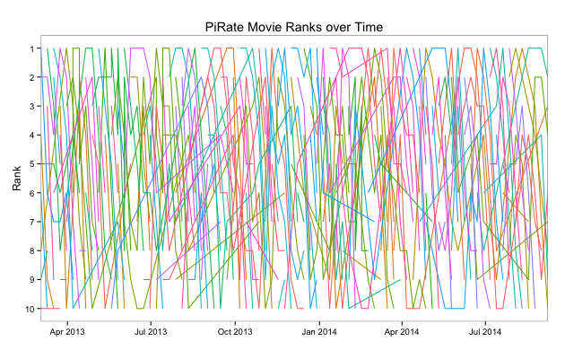
Complete. Chaos. Even if we highlight certain movies and push others to the background it’s still a bit of a mess (select the picture to see a larger/longer chart):
# set the color for all the 'background' movies
drt <- combined %>%  select(Title, rank, date) %>% mutate(color="Not Selected")

# _somewhat_ arbitrary selection here
selected_titles <- c("Frozen",
                     "Captain America: The Winter Soldier",
                     "The Amazing Spider-Man 2",
                     "Star Trek Into Darkness",
                     "The Hobbit: An Unexpected Journey",
                     "The Hobbit: The Desolation of Smaug")

# we'll use the Title field for the color factor levels
drt[drt$Title %in% selected_titles,]$color <- drt[drt$Title %in% selected_titles,]$Title
drt$color <- factor(drt$color, levels = c("Not Selected", selected_titles), ordered = TRUE)

# by using a manual color scale and our new factor variable, we can
# highlight the few selected_titles. You'll need to use a different RColorBrewer scale
# if you up the # of movies too much, tho.

ggplot(drt, aes(x=date, y=rank, group=Title)) +
  geom_line(aes(color=color)) +
  scale_x_date(expand=c(0,0)) +
  scale_y_reverse(breaks=c(10:1)) +
  scale_color_manual(values=c("#e7e7e7", brewer.pal(length(selected_titles), "Dark2")), name="Movie") +
  theme_bw() + theme(legend.position="bottom", legend.direction="vertical", panel.grid=element_blank())
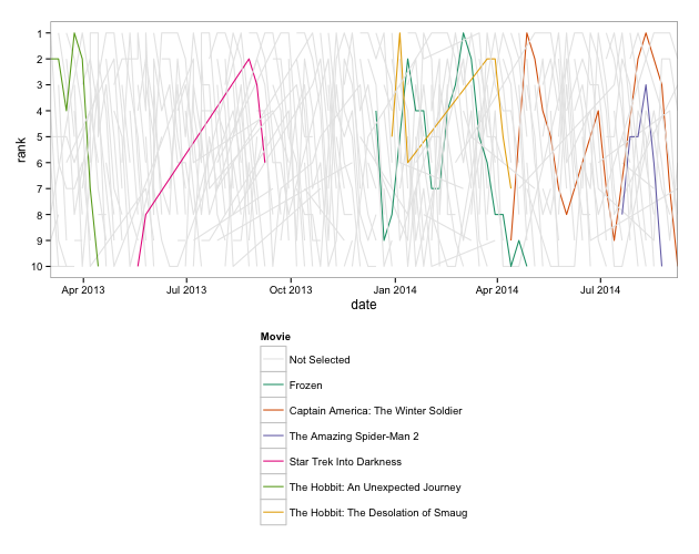
We’d have to do that interactively (via Shiny or perhaps an export to D3) to make much sense out of it.
Let’s see if a “small multiples” approach gets us any further. We’ll plot each movie’s rank over time and order them by the number of weeks they were on the piRate charts. Now, there are quite a number of movies in this data set (length(unique(combined$Title)) gives me 217 for the rda on github), so first we’ll see what the distribution by # weeks on the chaRts looks like:
combined %>% select(Title, freq) %>%
  unique %>% ggplot(aes(x=freq)) +
  geom_histogram(aes(fill=freq)) +
  labs(x="# Weeks on ChaRts", y="Movie count") +
  theme_bw() +
  theme(legend.position="none")
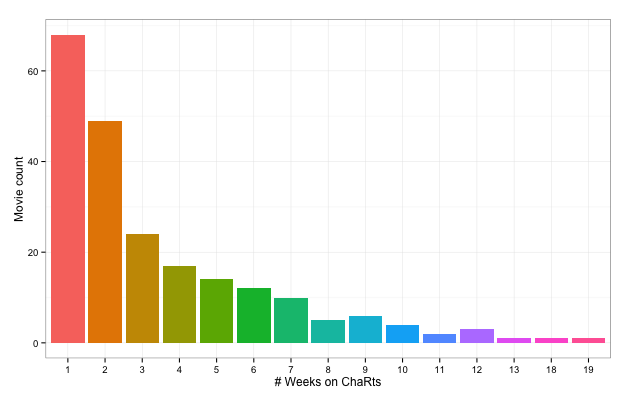
There are quite a few “one/two-hit-wonders/plunders” so we’ll make the cutoff for our facets at 4+ weeks (which also gives us just enough ColorBrewer colors to work with). Some of the movie titles are quite long, and I think it makes sense to label each facet by the movie name, so first we’ll abbreviate the names and then make the plot, coloring the facets by # of weeks on the piRate chaRts (select chart for larger version):
# abbreviate the titles
combined$short.title <- abbreviate(combined$Title, minlength=14)

# order the new short.title factor by # wks on charts
combined$short.title <- factor(combined$short.title, levels=unique(combined$short.title[order(-combined$freq)], ordered=TRUE))

gg <- ggplot(data=combined %>% filter(as.numeric(freq)>=4), aes(x=date, y=rank, group=short.title))
gg <- gg + geom_segment(aes(x=date, xend=date, y=10, yend=rank, color=freq), size=0.25)
gg <- gg + geom_point(aes(color=freq), size=1)
gg <- gg + scale_color_brewer(palette = "Paired", name="# Weeks on PiRate ChaRts")
gg <- gg + scale_fill_brewer(palette = "Paired", name="# Weeks on PiRate ChaRts")
gg <- gg + scale_y_reverse(label=floor)
gg <- gg + labs(x="", y="", title="PiRated Weekly Movie Rankings : March 2013 - September 2014")
gg <- gg + facet_wrap(~short.title, ncol=6)
gg <- gg + theme_bw()
gg <- gg + theme(text=element_text(family="Gotham Medium"))
gg <- gg + theme(strip.background=element_blank())
gg <- gg + theme(panel.grid=element_blank())
gg <- gg + theme(axis.ticks.x=element_blank())
gg <- gg + theme(axis.text.x=element_blank())
gg <- gg + theme(legend.position="top")
gg
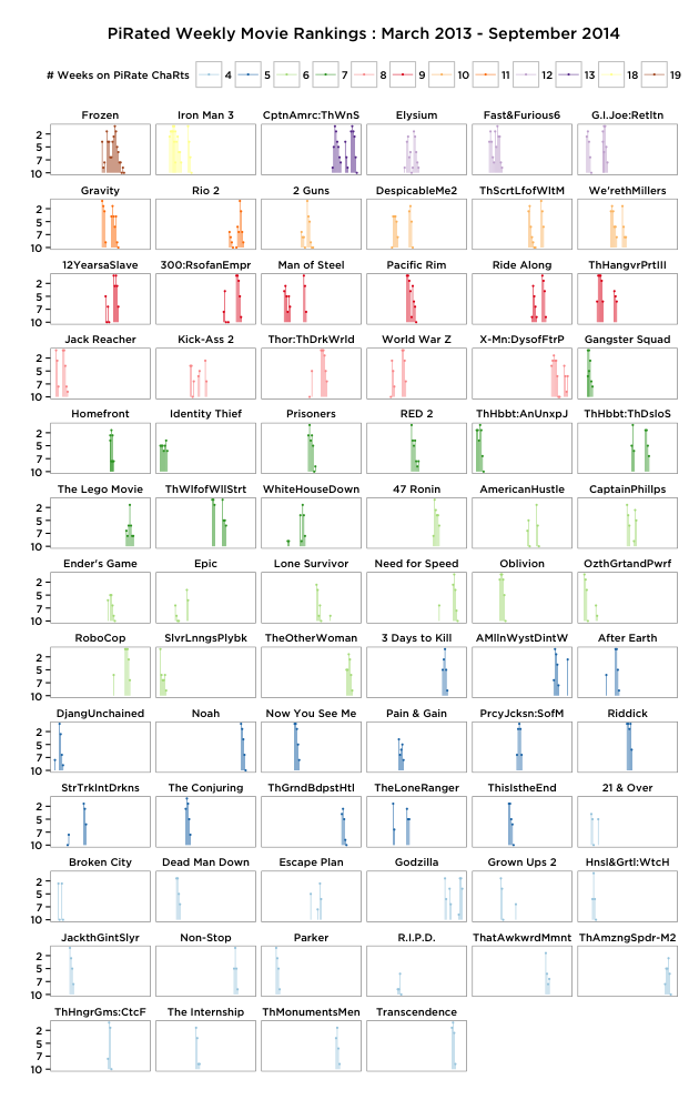
The title of the post should make a bit more sense now as Frozen is the clear “winner” (can it be winning to be the one with the most unrealized revenue?). This visual inspection alone sheds some light on piRate habits, but we’ll need more data to confirm any nascent hypotheses.
Augmenting our PiRate Data
So far, we know movie frequency (# weeks on the chaRts) and rank over time. We could definitely use more movie metadata. Since we have the IMDb movie id from the TorrentFreak posts, we can use the Open Movie Database API (OMDb) by Brian Fritz to retrieve a great deal more information, including many details from Rotten Tomatoes. This time we use httr and jsonlite to process the API queries. The API response is clean enough to do a very quick conversion:
# call out to the OMDB API for rotten tomatoes and other bits of info
getOMDBInfo <- function(imdb.ids) {

  do.call("rbind", pblapply(unique(imdb.ids), function(imdb.id) {

    dat <- GET(sprintf("https://www.omdbapi.com/?i=%s&tomatoes=TRUE", imdb.id))
    data.frame(fromJSON(content(dat, as="text")), stringsAsFactors=FALSE)

  }))

}

# makes 10K 10000 (etc)
# adapted from https://stackoverflow.com/a/15015037/1457051
currencyToNumeric <- function(vector) {

  vector <- as.character(vector) %>% gsub("(\\$|,| )", "", .) %>% as.numeric

  k_positions <- grep("K", vector, ignore.case=TRUE)
  result[k_positions] <- as.numeric(gsub("K", "", vector[k_positions])) * 1000

  m_positions <- grep("M", vector, ignore.case=TRUE)
  result[m_positions] <- as.numeric(gsub("M", "", vector[m_positions])) * 1000000

  return(result)

}

cleanUpOMDB <- function(omdb) {

  omdb$imdbVotes <- as.numeric(gsub(",", "", omdb$imdbVotes))
  omdb$tomatoUserReviews <- as.numeric(gsub(",", "", omdb$tomatoUserReviews))

  # only convert some columns to numeric

  for(col in c("Metascore", "imdbRating", "tomatoUserRating",
               "tomatoMeter", "tomatoRating", "tomatoReviews",
               "tomatoFresh", "tomatoRotten", "tomatoUserMeter")) {
    omdb[,col] <- as.numeric(omdb[,col])
  }

  omdb$BoxOffice <- currencyToNumeric(omdb$BoxOffice)

  omdb$DVD <- as.Date(omdb$DVD, format="%d %b %Y")
  omdb$Released <- as.Date(omdb$Released, format="%d %b %Y")

  omdb$Rated <- factor(omdb$Rated)
  omdb$Runtime <- as.numeric(gsub("\ *min", "", omdb$Runtime))

  omdb

}

cleanUpOMDB(getOMDBInfo(combined$imdb.id))
combined <- merge(combined, omdb, by.x="imdb.id", by.y="imdbID")
Even the OMDb data needs some cleanup and conversion to proper R data types. We also convert 10m to 10000000 so we can actually use the revenue metadata. If you inspect the combined data frame, you’ll see there are missing and/or errant bits of information, even from the cleaned OMDb data. We need to fill in DVD release dates and fix the MPAA ratings for a few titles. Again, doing this programmatically (vs by hand) helps make this process usable at a later date if we need to re-scrape the data.
combined[combined$Title=="12 Years a Slave",]$DVD <- as.Date("2014-03-04")
combined[combined$Title=="Breakout",]$DVD <- as.Date("2013-09-17")
combined[combined$Title=="Dead in Tombstone",]$DVD <- as.Date("2013-10-22")
combined[combined$Title=="Dhoom: 3",]$DVD <- as.Date("2014-04-15")
combined[combined$Title=="Ender's Game",]$DVD <- as.Date("2014-02-11")
combined[combined$Title=="Epic",]$DVD <- as.Date("2013-08-20")
combined[combined$Title=="Iron Man: Rise of Technovore",]$DVD <- as.Date("2013-04-16")
combined[combined$Title=="Once Upon a Time in Mumbai Dobaara!",]$DVD <- as.Date("2013-10-26")
combined[combined$Title=="Redemption",]$DVD <- as.Date("2013-09-24")
combined[combined$Title=="Rise of the Guardians",]$DVD <- as.Date("2013-03-12")
combined[combined$Title=="Scavengers",]$DVD <- as.Date("2013-09-03")
combined[combined$Title=="Shootout at Wadala",]$DVD <- as.Date("2013-06-15")
combined[combined$Title=="Sleeping Beauty",]$DVD <- as.Date("2012-04-10")
combined[combined$Title=="Son of Batman",]$DVD <- as.Date("2014-05-06")
combined[combined$Title=="Stand Off",]$DVD <- as.Date("2013-03-26")
combined[combined$Title=="Tarzan",]$DVD <- as.Date("2014-08-05")
combined[combined$Title=="The Hangover Part III",]$DVD <- as.Date("2013-10-08")
combined[combined$Title=="The Wicked",]$DVD <- as.Date("2013-04-30")
combined[combined$Title=="Welcome to the Punch",]$DVD <- as.Date("2013-05-08")

# some ratings were missing and/or incorrect
combined[combined$Title=="Bad Country",]$Rated <- "R"
combined[combined$Title=="Breakout",]$Rated <- "R"
combined[combined$Title=="Dhoom: 3",]$Rated <- "Unrated"
combined[combined$Title=="Drive Hard",]$Rated <- "PG-13"
combined[combined$Title=="Once Upon a Time in Mumbai Dobaara!",]$Rated <- "Unrated"
combined[combined$Title=="Scavengers",]$Rated <- "PG-13"
combined[combined$Title=="Shootout at Wadala",]$Rated <- "Unrated"
combined[combined$Title=="Sleeping Beauty",]$Rated <- "Unrated"
combined[combined$Title=="Sparks",]$Rated <- "Unrated"
combined[combined$Title=="Street Fighter: Assassin's Fist",]$Rated <- "Unrated"
combined[combined$Title=="The Colony",]$Rated <- "R"
combined[combined$Title=="The Last Days on Mars",]$Rated <- "R"
combined[combined$Title=="The Physician",]$Rated <- "PG-13"

# normalize the ratings (Unrated == Not Rated)
combined[combined$Rated=="Not Rated", "Rated"] <- "Unrated"
combined$Rated <- factor(as.character(combined$Rated))
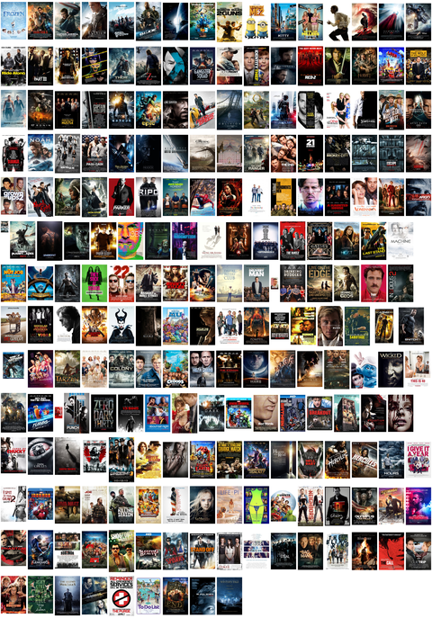
We now have quite a bit of data to try to find some reason for all this piRacy (once more, a reminder to use the github repo to reproduce this R project). We can have some fun, first, and use R (with some help from ImageMagick) to grab all the movie posters and make a montage out of them in decending order (based on # weeks on the pirate charts):
downloadPosters <- function(combined, .progress=TRUE) {

  posters <- combined %>% select(imdb.id, Poster) %>% unique

  invisible(mapply(function(id, img) {
    dest_file <- sprintf("data/posters/%s.jpg", id)
    if (!file.exists(dest_file)) {
      if (.progress) {
        message(img)
        GET(img, write_disk(dest_file), progress("down"))
      } else {
        GET(img, write_disk(dest_file))
      }
    }
  }, posters$imdb.id, posters$Poster))

}

downloadPosters(combined)

descending_ids <- combined %>% arrange(desc(freq)) %>% select(imdb.id) %>% unique %>% .$imdb.id

system(paste("montage ",
             paste(sprintf("data/posters/%s.jpg", descending_ids), collapse=" "),
             " -geometry +10+23 data/montage.png"))

system("convert data/montage.png -resize 480 data/montage.png")
Thirty-six movies made it to “#1” in the piRate top 10 charts, lets see if there was anything common across these posters for them. We’ll plot the posters with their RGB histograms and order them by box office receipts (you’ll definitely want to grab the larger version from the pop-up image, perhaps even download it):
# get all the #1 hits & sort them by box office receipts
number_one <- combined %>% group_by(Title) %>% filter(rank==1, rating==max(rating)) %>% select(Title, short.title, imdb.id, rank, rating, BoxOffice) %>% ungroup %>% unique
number_one <- number_one[complete.cases(number_one),] %>% arrange(desc(BoxOffice))

# read in all their poster images
posters <- sapply(number_one$imdb.id, function(x) readJpeg(sprintf("data/posters/%s.jpg", x)))

# calculate the max bin count so we can normalize the histograms across RGB plots & movies
hist_max <- max(sapply(number_one$imdb.id, function(x) {
  max(hist(posters[[x]][,,1], plot=FALSE, breaks=seq(from=0, to=260, by=10))$counts,
      hist(posters[[x]][,,2], plot=FALSE, breaks=seq(from=0, to=260, by=10))$counts,
      hist(posters[[x]][,,3], plot=FALSE, breaks=seq(from=0, to=260, by=10))$counts)
}))

# plot the histograms with the poster, labeling with short title and $
n<-nrow(dat)
png("data/posters/histograms.png", width=3600, height=1800)
plot.new()
par(mar=rep(2, 4))
par(mfrow=c(n/3, 12))
for (i in 1:12) {
  for (j in 1:3) {
    plot(posters[[i*j]])
    hist(posters[[i*j]][,,1], col="red", xlab = "", ylab = "", main="", breaks=seq(from=0, to=260, by=10), ylim=c(0,hist_max))
    hist(posters[[i*j]][,,2], col="green", xlab = "", ylab = "", main=sprintf("%s - %s", dat[i*j,]$short.title, dollar(dat[i*j,]$BoxOffice)), breaks=seq(from=0, to=260, by=10), ylim=c(0,hist_max))
    hist(posters[[i*j]][,,3], col="blue", xlab = "", ylab = "", main="", breaks=seq(from=0, to=260, by=10), ylim=c(0,hist_max))
  }
}
dev.off()
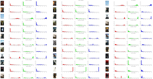
A few stand out as being very different, but there aren’t many true commonalities between these sets of posters.
For reference, here’s what our data frame looks like so far:
str(combined)

## 'data.frame':    792 obs. of  40 variables:
##  $ Title            : chr  "12 Years a Slave" "12 Years a Slave" "12 Years a Slave" "12 Years a Slave" ...
##  $ imdb.id          : chr  "tt2024544" "tt2024544" "tt2024544" "tt2024544" ...
##  $ date             : Date, format: "2014-01-19" "2014-02-23" "2014-03-16" "2014-03-02" ...
##  $ movie            : chr  "12 Years a Slave" "12 Years a Slave" "12 Years a Slave" "12 Years a Slave" ...
##  $ rank             : num  7 1 3 3 10 1 7 5 10 10 ...
##  $ rating           : num  8.6 8.4 8.4 8.4 8.6 8.4 8.4 8.6 8.6 6.2 ...
##  $ Year             : chr  "2013" "2013" "2013" "2013" ...
##  $ Rated            : Factor w/ 5 levels "G","PG","PG-13",..: 4 4 4 4 4 4 4 4 4 4 ...
##  $ Released         : Date, format: "2013-11-08" "2013-11-08" "2013-11-08" "2013-11-08" ...
##  $ Runtime          : num  134 134 134 134 134 134 134 134 134 93 ...
##  $ Genre            : chr  "Biography, Drama, History" "Biography, Drama, History" "Biography, Drama, History" "Biography, Drama, History" ...
##  $ Director         : chr  "Steve McQueen" "Steve McQueen" "Steve McQueen" "Steve McQueen" ...
##  $ Writer           : chr  "John Ridley (screenplay), Solomon Northup (based on \"Twelve Years a Slave\" by)" "John Ridley (screenplay), Solomon Northup (based on \"Twelve Years a Slave\" by)" "John Ridley (screenplay), Solomon Northup (based on \"Twelve Years a Slave\" by)" "John Ridley (screenplay), Solomon Northup (based on \"Twelve Years a Slave\" by)" ...
##  $ Actors           : chr  "Chiwetel Ejiofor, Dwight Henry, Dickie Gravois, Bryan Batt" "Chiwetel Ejiofor, Dwight Henry, Dickie Gravois, Bryan Batt" "Chiwetel Ejiofor, Dwight Henry, Dickie Gravois, Bryan Batt" "Chiwetel Ejiofor, Dwight Henry, Dickie Gravois, Bryan Batt" ...
##  $ Plot             : chr  "In the antebellum United States, Solomon Northup, a free black man from upstate New York, is abducted and sold into slavery." "In the antebellum United States, Solomon Northup, a free black man from upstate New York, is abducted and sold into slavery." "In the antebellum United States, Solomon Northup, a free black man from upstate New York, is abducted and sold into slavery." "In the antebellum United States, Solomon Northup, a free black man from upstate New York, is abducted and sold into slavery." ...
##  $ Language         : chr  "English" "English" "English" "English" ...
##  $ Country          : chr  "USA, UK" "USA, UK" "USA, UK" "USA, UK" ...
##  $ Awards           : chr  "Won 3 Oscars. Another 204 wins & 192 nominations." "Won 3 Oscars. Another 204 wins & 192 nominations." "Won 3 Oscars. Another 204 wins & 192 nominations." "Won 3 Oscars. Another 204 wins & 192 nominations." ...
##  $ Poster           : chr  "https://ia.media-imdb.com/images/M/MV5BMjExMTEzODkyN15BMl5BanBnXkFtZTcwNTU4NTc4OQ@@._V1_SX300.jpg" "https://ia.media-imdb.com/images/M/MV5BMjExMTEzODkyN15BMl5BanBnXkFtZTcwNTU4NTc4OQ@@._V1_SX300.jpg" "https://ia.media-imdb.com/images/M/MV5BMjExMTEzODkyN15BMl5BanBnXkFtZTcwNTU4NTc4OQ@@._V1_SX300.jpg" "https://ia.media-imdb.com/images/M/MV5BMjExMTEzODkyN15BMl5BanBnXkFtZTcwNTU4NTc4OQ@@._V1_SX300.jpg" ...
##  $ Metascore        : num  97 97 97 97 97 97 97 97 97 44 ...
##  $ imdbRating       : num  8.2 8.2 8.2 8.2 8.2 8.2 8.2 8.2 8.2 6.2 ...
##  $ imdbVotes        : num  236225 236225 236225 236225 236225 ...
##  $ Type             : chr  "movie" "movie" "movie" "movie" ...
##  $ tomatoMeter      : num  NA NA NA NA NA NA NA NA NA 59 ...
##  $ tomatoImage      : chr  "N/A" "N/A" "N/A" "N/A" ...
##  $ tomatoRating     : num  NA NA NA NA NA NA NA NA NA 5.7 ...
##  $ tomatoReviews    : num  NA NA NA NA NA NA NA NA NA 37 ...
##  $ tomatoFresh      : num  NA NA NA NA NA NA NA NA NA 22 ...
##  $ tomatoRotten     : num  NA NA NA NA NA NA NA NA NA 15 ...
##  $ tomatoConsensus  : chr  "N/A" "N/A" "N/A" "N/A" ...
##  $ tomatoUserMeter  : num  NA NA NA NA NA NA NA NA NA 46 ...
##  $ tomatoUserRating : num  NA NA NA NA NA NA NA NA NA 3.1 ...
##  $ tomatoUserReviews: num  NA NA NA NA NA ...
##  $ DVD              : Date, format: "2014-03-04" "2014-03-04" "2014-03-04" "2014-03-04" ...
##  $ BoxOffice        : num  NA NA NA NA NA NA NA NA NA NA ...
##  $ Production       : chr  "N/A" "N/A" "N/A" "N/A" ...
##  $ Website          : chr  "N/A" "N/A" "N/A" "N/A" ...
##  $ Response         : chr  "True" "True" "True" "True" ...
##  $ short.title      : Factor w/ 217 levels "Frozen","Iron Man 3",..: 13 13 13 13 13 13 13 13 13 150 ...
##  $ freq             : Factor w/ 15 levels "1","2","3","4",..: 9 9 9 9 9 9 9 9 9 1 ...
Searching for Data TReasuRe
![]() We don’t have a full movie corpus and we don’t even have a full piRate movie corups, just the “top 10“‘s. So, we’ll take a bit more pragmatic approach to seeing what makes for fandom in the realm of the scurvy dogs and continue our treasure hunt with some additional exploratory data analysis (EDA). Let’s see what the distributions look like for some of our new categorical and continuous variables:
We don’t have a full movie corpus and we don’t even have a full piRate movie corups, just the “top 10“‘s. So, we’ll take a bit more pragmatic approach to seeing what makes for fandom in the realm of the scurvy dogs and continue our treasure hunt with some additional exploratory data analysis (EDA). Let’s see what the distributions look like for some of our new categorical and continuous variables:
# we'll be doing this again, so wrap it in a function
movieRanges <- function(movies, title="") {

  comb <- movies %>%
    select(short.title, rank, rating, Rated, Runtime, Metascore, imdbRating, imdbVotes,
           tomatoMeter, tomatoRating, tomatoReviews, tomatoFresh, tomatoRotten, BoxOffice) %>%
    group_by(short.title) %>% filter(row_number()==1) %>% ungroup

  comb$Rated <- as.numeric(comb$Rated)

  comb <- data.frame(short.title=as.character(comb$short.title), scale(comb[-1]))

  comb_melted <- comb %>% melt(id.vars=c("short.title"))

  cols <- colnames(comb)[-1]

  for(x in cols) {
    x <- as.character(x)
    y <- range(as.numeric(movies[, x]), na.rm=TRUE)
    comb_melted$variable <- gsub(x, sprintf("%s\n[%s:%s]", x,
                                            prettyNum(floor(y[1]), big.mark=",", scientific=FALSE),
                                            prettyNum(floor(y[2]), big.mark=",", scientific=FALSE)),
                                            as.character(comb_melted$variable))
  }

  gg <- comb_melted %>% ggplot(aes(x=variable, y=value, group=variable, fill=variable))
  gg <- gg + geom_violin()
  gg <- gg + coord_flip()
  gg <- gg + labs(x="", y="")
  gg <- gg + theme_bw()
  gg <- gg + theme(legend.position="none")
  gg <- gg + theme(panel.grid=element_blank())
  gg <- gg + theme(panel.border=element_blank())
  gg <- gg + theme(axis.text.x=element_blank())
  gg <- gg + theme(axis.text.y=element_text(size=20))
  gg <- gg + theme(axis.ticks.x=element_blank())
  gg <- gg + theme(axis.ticks.y=element_blank())
  if (title != "") { gg <- gg + labs(title=title) }
  gg

}

movieRanges(combined, "All Top 10 PiRate Movies")
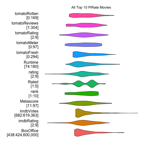
Violin plots are mostly just prettier version of boxplots and which encode the shape of the density mass function. This orchestral view lets us compare each variable visually. IMDb votes tracks with Box Office receipts, but there are no indicators of anything truly common about these movies. It was still my belief, however, that there had to be something that got and kept these movies on the PiRate Top 10 lists.
A look at movie genres does yeild some interesting findings as we see that top downloads are heavily weighted towards Comedy and Action, Adventure, Sci-Fi:
genre_table %>% arrange(desc(Count)) %>% head(10)

##                           Genre Count
## 1                        Comedy    18
## 2     Action, Adventure, Sci-Fi    11
## 3          Action, Crime, Drama     9
## 4       Action, Crime, Thriller     9
## 5  Animation, Adventure, Comedy     8
## 6         Action, Comedy, Crime     7
## 7        Crime, Drama, Thriller     6
## 8    Action, Adventure, Fantasy     5
## 9       Action, Drama, Thriller     5
## 10                       Horror     5

gg1 <- ggplot(genre_table, aes(xend=reorder(Genre, Count), yend=Count))
gg1 <- gg1 + geom_segment(aes(x=reorder(Genre, Count), y=0))
gg1 <- gg1 + geom_point(aes(x=reorder(Genre, Count), y=Count))
gg1 <- gg1 + scale_y_continuous(expand=c(0,0.5))
gg1 <- gg1 + labs(x="", y="", title="Movie counts by full genre classification")
gg1 <- gg1 + coord_flip()
gg1 <- gg1 + theme_bw()
gg1 <- gg1 + theme(panel.grid=element_blank())
gg1 <- gg1 + theme(panel.border=element_blank())
gg1
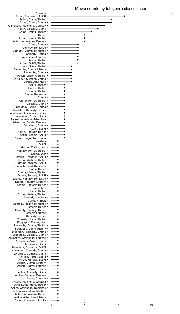
If we breakdown the full, combined genre into component parts, however, a slightly different pattern emerges:
single_genres <-  as.data.frame(table(unlist(strsplit(genre_table$Genre, ",\ *"))), stringsAsFactors=FALSE)
colnames(single_genres) <- c("Genre", "Count")
gg1 <- ggplot(single_genres, aes(xend=reorder(Genre, Count), yend=Count))
gg1 <- gg1 + geom_segment(aes(x=reorder(Genre, Count), y=0))
gg1 <- gg1 + geom_point(aes(x=reorder(Genre, Count), y=Count))
gg1 <- gg1 + scale_y_continuous(expand=c(0,0.5))
gg1 <- gg1 + labs(x="", y="")
gg1 <- gg1 + coord_flip()
gg1 <- gg1 + theme_bw()
gg1 <- gg1 + theme(panel.grid=element_blank())
gg1 <- gg1 + theme(panel.border=element_blank())
gg1
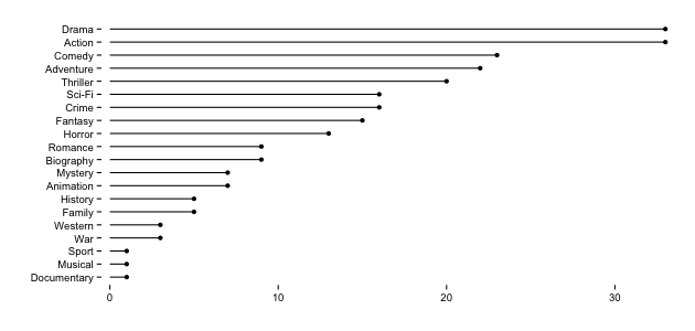
But, there are some commonalities between the two lists and there are definitely some genres & genre-components that rank higher, so we’ve at least got one potential indicator as to what gets you on the list. The other text fields did not yield much insight (unsurprisingly the movies gravitate towards the English language and being made in the USA), but others might have more luck.
Staying PoweR
If genre is one of the indicators that gets you on the list, what keeps you there? The presence of all the cam rips in the movie titles gave me the idea to see if there was a pattern to these movies getting into the top 10 based on date. I went back to my facet plot and decided to take a look at the movie release dates and DVD release dates by superimposing the time frames for each onto the facet graph:
gg <- ggplot(data=combined %>% filter(as.numeric(freq)>=4, !is.na(DVD)), aes(x=date, y=rank, group=short.title))
gg <- gg + geom_rect(aes(xmin=Released, xmax=DVD, ymin=0, ymax=10), fill="#dddddd", alpha=0.25)
gg <- gg + geom_segment(aes(x=Released, xend=Released, y=0, yend=10), color="#7f7f7f", size=0.125)
gg <- gg + geom_segment(aes(x=DVD, xend=DVD, y=0, yend=10), color="#7f7f7f", size=0.125)
gg <- gg + geom_segment(aes(x=date, xend=date, y=10, yend=rank, color=freq), size=0.25)
gg <- gg + geom_point(aes(color=freq), size=1)
gg <- gg + scale_color_brewer(palette = "Paired", name="# Weeks on PiRate ChaRts")
gg <- gg + scale_fill_brewer(palette = "Paired", name="# Weeks on PiRate ChaRts")
gg <- gg + scale_y_reverse(label=floor)
gg <- gg + labs(x="", y="", title="PiRated Weekly Movie Rankings : March 2013 - September 2014")
gg <- gg + facet_wrap(~short.title, ncol=6)
gg <- gg + theme_bw()
gg <- gg + theme(text=element_text(family="Gotham Medium"))
gg <- gg + theme(strip.background=element_blank())
gg <- gg + theme(panel.grid=element_blank())
gg <- gg + theme(axis.ticks.x=element_blank())
gg <- gg + theme(axis.text.x=element_blank())
gg <- gg + theme(legend.position="top")
gg
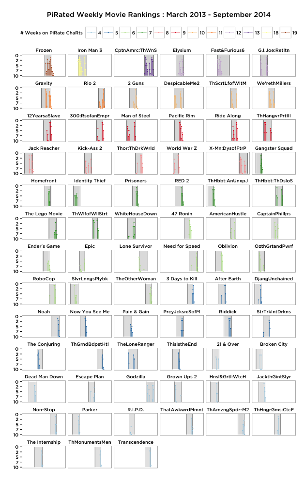
Now we’re getting somewhere. It seems that a movie hits the top charts right on opening day and continues on the charts (most of the time) until there’s a DVD release. This isn’t true for all of the movies, so let’s see which ones had longer runs than their DVD release dates (excluding ones that had only 1 extra week for post brevity):
beyond.dvd <- combined %>%
  group_by(Title) %>%
  summarise(n=sum(date > DVD)) %>%
  arrange(desc(n)) %>%
  filter(!is.na(n) & n>1)

beyond.dvd

## Source: local data frame [26 x 2]
##
##                                Title n
## 1                        Pacific Rim 7
## 2                             Frozen 6
## 3                          Divergent 5
## 4                             2 Guns 4
## 5                            Gravity 4
## 6  The Hobbit: An Unexpected Journey 4
## 7                   12 Years a Slave 3
## 8                     3 Days to Kill 3
## 9                           47 Ronin 3
## 10                              Argo 3
## 11                      Ender's Game 3
## 12                    Now You See Me 3
## 13                          Oblivion 3
## 14                       Pain & Gain 3
## 15                             RED 2 3
## 16          The Grand Budapest Hotel 3
## 17            300: Rise of an Empire 2
## 18                    Gangster Squad 2
## 19                      Jack Reacher 2
## 20                         Prisoners 2
## 21                        Ride Along 2
## 22                   The Other Woman 2
## 23           The Wolf of Wall Street 2
## 24                   This Is the End 2
## 25              Thor: The Dark World 2
## 26                       World War Z 2
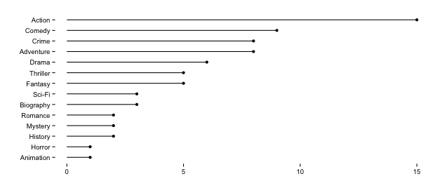
Pacific Rim was on the Top 10 PiRate ChaRts for 7 weeks past it’s DVD release date and beat Frozen O_o. Just by looking at the diversity of the titles, I’m skeptical of whether there are commonalities (beyond a desperate and cheapskate public) amongst these movies, but we’ll compare their sub-genres components (the full genre’s are almost evenly spread):
and their distributions against the previous ones (select the plot for larger version):
combined.beyond <- combined %>% group_by(Title) %>% mutate(weeks.past=sum(date>DVD)) %>% filter(date > DVD) %>% ungroup
grid.arrange(movieRanges(combined, "All Top 10 PiRate Movies"),
             movieRanges(combined.beyond, "Still in Top 10 Charts After\nPiRated AfteR DVD Release"), ncol=2)
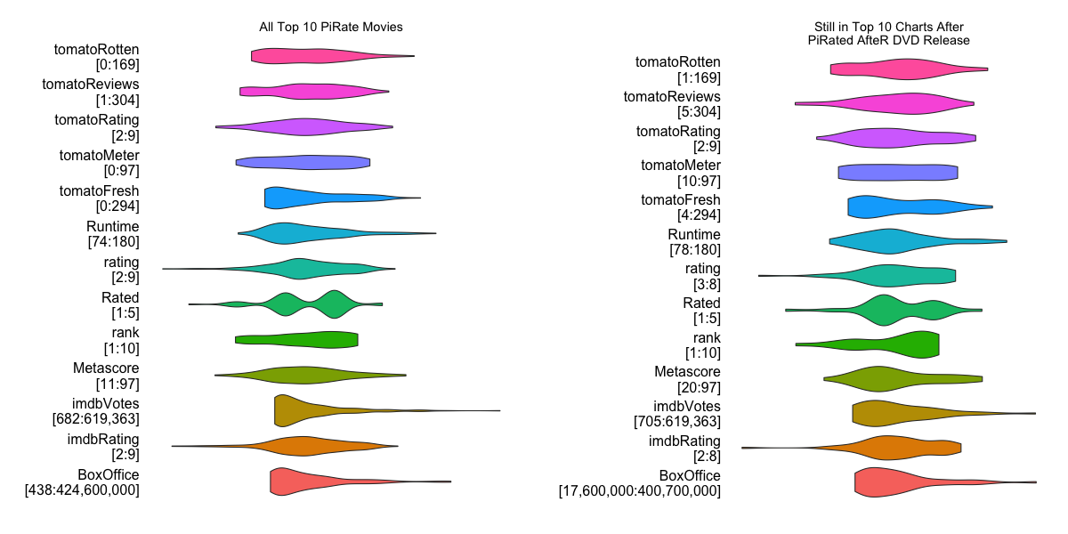
Some ranges are tighter and we can see some movement in the MPAA ratings, but no major drivers apart from Action & Comedy.
Conclusion & Next Steps
![]() We didn’t focus on all movies or even all piRated movies, just the ones in the TorrentFreak Top 10 list. I think adding in more diverse observations to the population would have helped identify some other key elements (besides questionalbe taste & frugality) for both what is pirated and why it may or may not land in the top 10. We did see a pretty clear pattern to the duration on the charts and some genres folks gravitate towards (though this could be due more to the fact that studios produce more of one genre than another throughout the year). It would seem from the last facet plot that Hollywood might be able to make a few more benjamins if they found some way to capitalize on the consumer’s desire to see movies in the comfort of their own abodes during the delay between theater & DVD release.
We didn’t focus on all movies or even all piRated movies, just the ones in the TorrentFreak Top 10 list. I think adding in more diverse observations to the population would have helped identify some other key elements (besides questionalbe taste & frugality) for both what is pirated and why it may or may not land in the top 10. We did see a pretty clear pattern to the duration on the charts and some genres folks gravitate towards (though this could be due more to the fact that studios produce more of one genre than another throughout the year). It would seem from the last facet plot that Hollywood might be able to make a few more benjamins if they found some way to capitalize on the consumer’s desire to see movies in the comfort of their own abodes during the delay between theater & DVD release.
You also now have a full data set (including CSV) of metadata about pirated movies to process on your own and try to make more sense out of than I did. You can also run the script to update the data and see if anything changes with time. With the movie poster download capability, you could even analyze popularity by colors used on the posters.
We hope you had fun on this year’s piRate journey with R!
Tweet