
By “Jay Jacobs (@jayjacobs)"
Mon 06 October 2014
|
tags:
blog,
r,
rstats,
-- (permalink)
This is part two of a three-part blog series on building a DGA classifier and it is split into the three phases of building a classifier: 1) Data preparation 2) Feature engineering and 3) Model selection (this post)
Back in part 1, we prepared the data and we are starting with a nice clean list of domains labeled as either legitimate (“legit”) or generated by an algorithm (“dga”). Then in part 2, we calculated various features which included length, entropy, several combinations of n-grams and finally a dictionary matching feature that calculated the percentage of characters that can be explained by dictionary words. Now we want to select a model and generate an algorithm to classify new domains. While we are doing that we will also double check how well each of the features we generated in part 2 perform. You should fully expect to remove several of our features during this step. If you’d like to follow along, you can grab the sampledga CSV directly or from R run the following code.
# this code will load up the compressed CSV from the dds website:
dataurl <- "https://datadrivensecurity.info/blog/data/2014/10/sampledga.csv.gz"
# create a gzip connection
con <- gzcon(url(dataurl))
# read in the (uncompressed) data
txt <- readLines(con)
# read in the text as a CSV
sampledga <- read.csv(textConnection(txt))
As we create an algorithm to classify, we have to answer a very, very important question… “How do we know this algorithm will perform well with data we haven’t seen yet?” All we have to work with is the data we have, so how can we get feedback about the data we haven’t seen? It would be a whole lot of work to go out and get a second labeled data set to test this against. The solution is a whole lot simpler: rather than use all of the data to generate the algorithm, you can set aside some samples to test how well the algorithm performs on data it hasn’t seen. These “test” samples will not be used to generate or “train” the algorithm so they will give you a fairly good sense of how well you are doing.
How we generate the “test” data and the “training” data can get a little
tricky on real data. The sample data in this example is fairly well
balanced with half being “legit” and the other half is “dga”. But if you
separate on the subclass you can see 4,948 samples are from alexa and
only 52 are from the opendns list of domains. If you were to randomly
separate the training from test data, you may get all the opendns
samples in one set and none in the other. To make sure we good
representation from each subclass we will do stratified random sampling,
meaning we will randomly assign each subclass to either the training or
test data to ensure even distribution. In order to do that quickly (and
most everything else in this step), we will leverage the caret
package.
An Brief Introduction to Caret
Directly from the package website, “The caret package (short for Classification And REgression Training) is a set of functions that attempt to streamline the process for creating predictive models.” It not only has an overwhelming list of models supported (over 150), it also has several supporting functions that will make this part of the process a whole lot easier. But it’s not enough to just install the caret package because it’s mostly just a wrapper. You’ll also have to install the package to support the model you are using. The huge benefit is that the way we will call different model is standardized and the results will be directly comparable. This is a huge advantage when selecting models.
Okay, let’s do a stratified sample based on the subclass using the caret package. I am going to split based on the subclass to ensure each source is represented evenly and I’m going to use 75% of the data to train the algorithm and hold out 25% of the data for testing later. As I create the training data, I will also remove fields we don’t need, for example the full hostname, domain and tld fields will not be used directly in the classification.
suppressPackageStartupMessages(library(caret))
# make this repeatable
set.seed(1492)
# if we pass in a factor, it will do the stratified sampling on it.
# this will return the row numbers to include in the training data
trainindex <- createDataPartition(sampledga$subclass, p=0.75, list=F)
# only train with these fields:
fields <- c("class", "length", "entropy", "dict", "gram345", "onegram",
            "twogram", "threegram", "fourgram", "fivegram")
# Now you can create a training and test data set
traindga <- sampledga[trainindex, fields]
# going to leave all the fields in the test data
testdga <- sampledga[-trainindex, ]
Just to verify, we can look the before and after samples of the subclass. You should expect 75% of each subclass to be in the training data.
summary(sampledga$subclass)

##        alexa cryptolocker          goz       newgoz      opendns
##         4948         1667         1667         1666           52

summary(sampledga$subclass[trainindex])

##        alexa cryptolocker          goz       newgoz      opendns
##         3711         1251         1251         1250           39
And now it gets a little complicated
Many of the models you can try have tuning parameters which are attributes of the model that don’t have a direct method of computing their value. For example, the Random Forest algorithm can be tuned for how many trees it grows in the forest (and no, I am not making up these terms). So the challenge with the tuning parameters is that we have to derive the best value for each parameter. Once again, the caret package will take care of most of that for you. For each model, you can tell the caret package to further split up the training data and do a process called cross-validation, which will hold out a portion of the training data to do internal checking and derive it’s best guess for the tuning parameters. To be sure you don’t allow a single bad split to influence the outcome, you can tell it to repeat it 5 times. There is a lot of stuff going into this code and I apologize for not explaining all of it. If you are really interested, you could read an introductory paper on the caret package.
I’m also going to run three different models here and compare them to
see which performs better. I’m going to compare a random
forest (rf), a support
vector machine
(svmRadial) and the C4.5
trees (it’s super fast).
Note that while the random forest and c4.5 models don’t care, the
support vector machine gets thrown off if the data is not preprocesed by
being centered and scaled. The support vector model also has an
additional tuneLength parameter that I needed to set.
# set up the training control attributes:
ctrl <- trainControl(method="repeatedcv",
                     repeats=5,
                     summaryFunction=twoClassSummary,
                     classProbs=TRUE)
rfFit <- train(class ~ .,
               data = traindga,
               metric="ROC",
               method = "rf",
               trControl = ctrl)
svmFit <- train(class ~ .,
                data = traindga,
                method = "svmRadial",
                preProc = c("center", "scale"),
                metric="ROC",
                tuneLength = 10,
                trControl = ctrl)
c45Fit <- train(class ~ .,
                data = traindga,
                method = "J48",
                metric="ROC",
                trControl = ctrl)
If you tried running these at home, you may have noticed those commands
were not exactly speedy (about 20 minutes for me). If you are working on
a multi-core system you could load up the doMC (multicore) package and
tell it how many cores to use with the registerDoMC() function. But be
warned, each core requires a lot of memory, and I run out of memory long
before I’m’ able to leverage all the cores.
But now you’ve got two models, in order to compare them, you can compare the resampling results it stored during the repeated cross-validation in the training.
resamp <- resamples(list(rf=rfFit, svm=svmFit, c45=c45Fit))
print(summary(resamp))

## Call:
## summary.resamples(object = resamp)
##
## Models: rf, svm, c45
## Number of resamples: 50
##
## ROC
##       Min. 1st Qu. Median   Mean 3rd Qu. Max. NA's
## rf  0.9982  0.9997 0.9999 0.9997  1.0000    1    0
## svm 0.9983  0.9993 0.9999 0.9996  1.0000    1    0
## c45 0.9901  0.9943 0.9972 0.9963  0.9986    1    0
##
## Sens
##       Min. 1st Qu. Median   Mean 3rd Qu. Max. NA's
## rf  0.9893  0.9947 0.9973 0.9959  0.9993    1    0
## svm 0.9787  0.9920 0.9947 0.9948  0.9973    1    0
## c45 0.9840  0.9947 0.9973 0.9951  0.9973    1    0
##
## Spec
##       Min. 1st Qu. Median   Mean 3rd Qu. Max. NA's
## rf  0.9813  0.9920 0.9960 0.9953  0.9973    1    0
## svm 0.9867  0.9947 0.9973 0.9955  0.9973    1    0
## c45 0.9867  0.9893 0.9947 0.9938  0.9973    1    0
Just looking at these numbers the SVM and random forest are close, the
C4.5 isn’t so close. It’s possible to test the differences with the
diff command and we see that the there is no significant difference
between the svm and rf model, but the c4.5 is significantly different
from both the rf and svm model (with a p-value of 4.629e-10 and
5.993e-10 respectively). With the decision between the random forest and
support vector machine, I am going with the random forest here. It’s a
little simpler to comprehend and explain and it’s less complicated
overall, either one would be fine though.
Now with just the random forest, let’s look at how the variables
contributed by using the varImp function (variable importance).
importance <- varImp(rfFit, scale=F)
plot(importance)
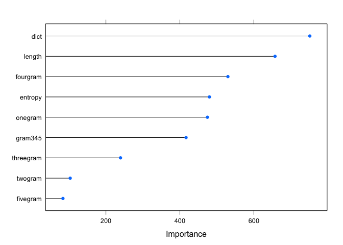
It’s no surprise that the dict feature is at the top here. We could
see the huge difference in the plot back in part 2. It’s interesting to
see the 2 and 5 n-gram at the bottom. Now we’ve got an iterative
process. We could drop a few variables and re-run, maybe add some back
in, and so on. All the while keeping an eye on this plot. After doing
this, I found I could (surprisingly) drop the entropy and all the
single values n-grams and just go with the gram345 feature (as Click
Security used) along with the length and dict features.
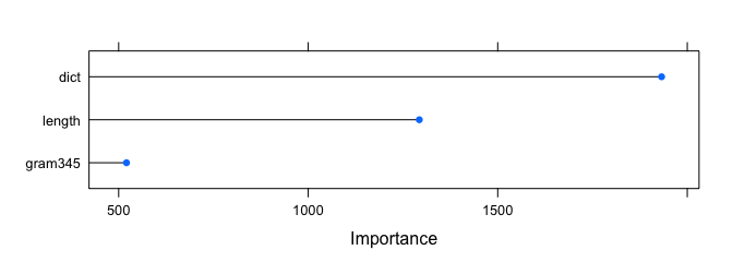
# we still have the trainindex value from before, so just trim
# the fields and re-run the random forest
fields <- c("class", "length", "dict", "gram345")
traindga <- sampledga[trainindex, fields]
rfFit2 <- train(class ~ .,
                data = traindga,
                metric="ROC",
                method = "rf",
                trControl = ctrl)

plot(varImp(rfFit2, scale=F))
And…
resamp <- resamples(list(rf1=rfFit, rf2=rfFit2))
diffs <- diff(resamp)
print(diffs$statistics$ROC$rf1.diff.rf2)

##
##  One Sample t-test
##
## data:  x
## t = 2.243, df = 49, p-value = 0.02948
## alternative hypothesis: true mean is not equal to 0
## 95 percent confidence interval:
##  3.419e-05 6.241e-04
## sample estimates:
## mean of x
## 0.0003291
Even though the model with all of the initial features is slightly better, the difference may be considered negligible (p-value of 0.02 on testing if they are different). Plus by cutting all of those features we are saving the time and effort to generate the features and classify them based on all those features. Depending on the environment the classifier is going to run, that improvement in speed may be worth the decrease in overall accuracy.
The confusion matrix
One other thing I do quite a bit of is look at the confusion matrix.
Remember we pulled out that test data so we could see how the model does
on “new” data? Well we can do that by looking at what’s called the
confusion matrix (see Dan Geer’s October “For Good Measure”
column for a nice
discussion of the concepts). With the test data you held out, you can
run the predict function on and then see how well the classification
performed by printing the confusion matrix:
pred <- predict(rfFit2, testdga)
print(confusionMatrix(pred, testdga$class))

## Confusion Matrix and Statistics
##
##           Reference
## Prediction  dga legit
##      dga   1242     5
##      legit    6  1245
##
##                Accuracy : 0.996
##                  95% CI : (0.992, 0.998)
##     No Information Rate : 0.5
##     P-Value [Acc > NIR] : <2e-16
##
##                   Kappa : 0.991
##  Mcnemar's Test P-Value : 1
##
##             Sensitivity : 0.995
##             Specificity : 0.996
##          Pos Pred Value : 0.996
##          Neg Pred Value : 0.995
##              Prevalence : 0.500
##          Detection Rate : 0.497
##    Detection Prevalence : 0.499
##       Balanced Accuracy : 0.996
##
##        'Positive' Class : dga
##
That’s pretty good, out of the 1,247 domains generated by a DGA, only 5 were mis-classified (looking at the first table in the output above), with a simliar ratio on the legitimate side. If you were curious, you could pull out the misclassified from the test data and see which domains failed to be correct. But all in all, this is a fairly accurate classifier!
This isn’t quite done though, now that you know what features to include
and what algorithm to train, you should go back to your original data
set and generate the final model on all the data. In order to use this
on data you haven’t seen yet, you would need to generate the features
you used in the final model (length, dict and gram345) and then run the
predict function with the algorithm generated with all of your labeled data.
Conclusion
As a final word and note of caution, it’s important to keep in mind the data used here and be very aware that any classifier is only as good as the training data. The training data used here included domains from the Cryptolocker and GOZ botnets. We should have a fairly high degree of confidence that this will do well classifying those two botnets from legitimate traffic, but we shouldn’t have the same confidence that this will apply to all domains generated from any current or future DGA. Instead, as new domains are observed and new botnets emerge, this process should be repeated with new training data.
Unfortunately I had to gloss over many, many points here. And if you’ve read through this post, you realize that feature engineering isn’t isolated from model selection and often exist in an iterative process. Overall though, hopefully this gave you a glimpse of the process for generating a classifier or least what went into building a DGA classifier.
Tweet