By “Jay Jacobs (@jayjacobs)"
Sun 16 November 2014 | tags: blog, r, rstats, -- (permalink)

SIRAcon, the annual conference for the Society of Information Risk Analysts was held September 9th and 10th. I was fortunate enough to not only attend, but I also spoke (on how to stop worrying and love math) and moderated a fantastic panel with Ali-Samad-Khan, Jack Jones and Doug Hubbard. It was a fantastic 2-day conference and not just because of the speakers. The small venue and schedule enabled multiple networking opportunities and side conversations. One of my conversation was with Doug Hubbard where the Rule of Five came up from his first book.

The “Rule of Five” states, “There is a 93.75% chance that the median of a population is between the smallest and largest values in any random sample of five from that population.” And even though the math on it is fairly easy, I found it much more fun to think through how to simulate it. There may be times when the math is either too complex (relative term, I know), but creating a simulation may be the only option.

Let’s think through this, first we will need a population and the median of that population. We will draw our population from a normal distribution, but it could be any type of distribution, since we are working with the median, it doesn’t matter.

set.seed(1)  # make it repeatable
pop <- rnorm(1000)  # generate the "population"
med <- median(pop) # calculate the median

Next, we will want to repeatedly draw 5 random samples from the population and check if the median from the population is in the range (between the minimum and maximum) of the 5 samples. According to to setup, we should expect 93.75% of the samples to contain the median.

ssize <- 100000 # how many trials to run
matched <- sapply(seq(ssize), function(i) {
  rg <- range(sample(pop, 5)) # get the range for 5 random samples
  ifelse(med>=rg[1] & med<=rg[2], TRUE, FALSE) # test if median in range
})
sum(matched)/ssize # proportion matched

## [1] 0.9383

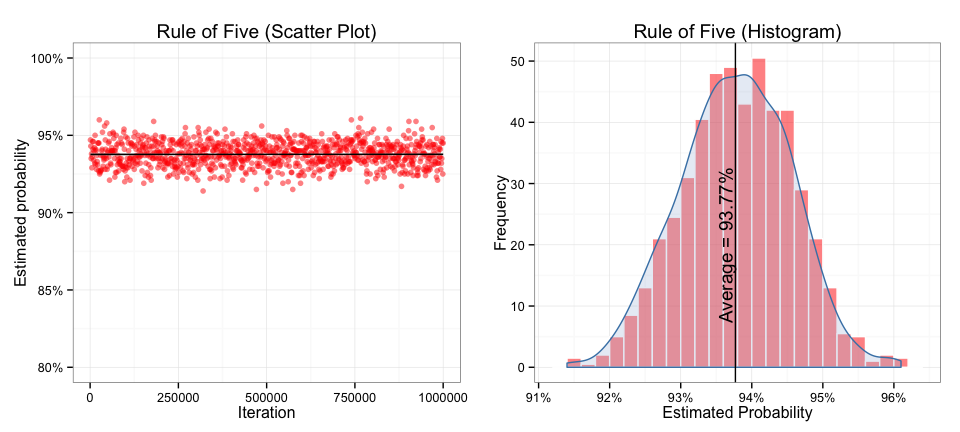
That’s pretty close to 93.75%, but what if we broke this up across multiple populations (and sizes) and used many iterations? Let’s create a simluation where we generate populations of varying sizes, capture a whole bunch of these and then plot the output.

# first set up a function to do the sampling
pickfive <- function(popsize, ssize) {
  pop <- rnorm(popsize)
  med <- median(pop)
  matched <- sapply(seq(ssize), function(i) {
     rg <- range(sample(pop, 5))
     ifelse(med>=rg[1] & med<=rg[2], TRUE, FALSE)
  })
  sum(matched)/ssize
}
# test it
pickfive(popsize=1000, ssize=100000)

## [1] 0.9381

Now we can create a loop to call the function over and over again.

# 1,000 to 1 million by a thousand
set.seed(1)
possible <- seq(1000, 1000000, by=1000)
output <- sapply(possible, pickfive, 5000) # takes a while
print(mean(output))

## [1] 0.9377

And we can visualize the variations in the samples:

There are so many interesting concepts being touched on here. First, this is a great example of the Law of Large Numbers — the more iterations we do, the closer to reality our estimation will be. Also, the results will form a normal distribution around the true answer, no matter what the underlying population looks like, that’s why taking the mean works. Finally, this also hints at a concept underlying many machine learning algorithms: combining multiple ‘weak predictors’ is more accurate than one (or handful) of strong predictors. By taking the mean of all our outputs (even the samples that are way off) we are using all the samples to derive a more accurate estimate of true value.

Oh yeah, the math…

The math here is so much simpler than all the stuff I did above (but so much less exciting). Since we talking about the median, 50% of the samples should be above and below the median value. This sets a coin-toss analogy: if we say heads is above the median and tails is below, what is the probability of flipping either 5 heads or 5 tails in a row? It is the same thing, we want to know the probability that all 5 of our samples will be above (or below) the median. The math is simply 50% to the power of 5 for getting either 5 tails or heads in row. So we can calculate it once and double it (once for heads, twice for tails). Then we want to know what the probability is of not getting heads, so we subtract it from 1.

# probability of getting 5 heads in a row
prob_of_heads <- 0.5 ^ 5  # == 0.03125

# probability of getting 5 heads or 5 tails in a row
prob_of_heads_or_tails <- 2 * prob_of_heads # == 0.0625

# probability of NOT getting 5 heads or tails in a row
rule_of_five <- (1 - prob_of_heads_or_tails)  # yup, 0.9375 or 93.75%

Or, if we want to wrap this whole discussion up into a single line of code:

print(1 - 2 * 0.5^5)

## [1] 0.9375

I told ya the math was easy! But simluations likes this are fun to do and come in handy if you don’t know (or can’t remember) the math. Plus with this, you should be to able to now go simulate the “Urn of Mystery” (chapter 3, 3rd edition of How to Measure Anything). Or better yet, use this skill of simulation to finally prove to yourself how the infamous Monte Hall problem actually works out like the math says it should.