By Bob Rudis (@hrbrmstr)
Tue 21 January 2014 | tags: maps, d3, map, cartography, -- (permalink)

(This series of posts expands on a topic presented in Chapter 5 of Data Driven Security : The Book)

Cartographers (map makers) and infosec professionals both have the unenviable task of figuring out the best way to communite complexity to a diverse audience. Maps hold an unwarranted place of privilege in the minds of viewers and they seem to have taken an equally unwarranted place of status when it comes to infosec folk wanting to show where “badness” comes from. More often than not, these malicious locations are displayed on a Google Map using Google’s maps API. Now, Google Maps is great for directions and managing specific physical waypoints, but they imply a level of precision that is just not there when attributing IP address malfeasnace. Plus, when you use Google Maps, you’re embedding a great deal of third-party code, user tracking and URL calls that just aren’t necessary when there are plenty of other ways to get the same points on a map; plus, if you don’t delve into the Google Maps API, you’re limited to a very meh representation of the globe.

This post kicks of a series that will cover the fundamentals of cartographic machinations and—at various points—show you how to make maps in D3 (and R/Python if time permits), all in a more accurate way than you can with Google Maps. The data we’ll use is from the marx data set in Jay’s “*Inspecting Internet Traffic” series. You’ll want to follow along until the final post as we’ll be covering the most important aspect of creating map visualizations: when not to use them.

The Making of a Map

Maps have three primary distinct attributes: scale, projection, and symbolic representation. Any (all, really) of those elements distort reality in some way. Scale distorts size and hides (or overemphasizes) detail. Projections take our very 3D world and mathematically flatten it onto a 2D canvas, requiring numerous tradeoffs between accuracy and readability. Symbols describe and distinguish geographic features and locations and guide viewers into knowing what bits are/aren’t relevant. In this post, we’re going to focus mainly on the projection and symbolic representation components, but we’ll touch a bit on scale as well.

The first thing we need to do is geolocate the honeypot data. There are real pitfalls when geolocating IP addresses that we cover fairly thoroughly in the book, so we’ll issue a caveat lector and move on to adding geographic information to the marx data set with a simple Python script that uses the MaxMind GeoLite2 database and corresponding Python API:

import csv
import geoip2.database

# yeah, despite having a nice long int, the city lookup function
# requires a string so we have to do this

def to_string(ip):
  return ".".join(map(lambda n: str(ip>>n & 0xFF), [24,16,8,0]))

# you'll need to download the city database and point this to it

reader = geoip2.database.Reader('GeoLite2-City.mmdb')

with open('marx.csv', 'rb') as marx:
  with open('marx-geo.csv', 'w') as f:
    flyreader = csv.reader(marx, delimiter=',', quotechar='"')
    for fly in flyreader:
      strIP = to_string(int(fly[2]))
      try: # sometimes the city function coughs up blood
        r = reader.city(strIP)
        f.write("%s%s,%s,%s,%s,%s,%s,%s,%s\n" % 
                                    (','.join(fly),
                                     strIP,
                                     r.country.iso_code,
                                     r.country.name, 
                                     r.subdivisions.most_specific.name,
                                     r.subdivisions.most_specific.iso_code,
                                     r.postal.code,
                                     r.location.latitude,
                                     r.location.longitude))
      except:
        f.write("%s%s,,,,,,,,\n" % (','.join(fly), strIP))

That will produce a new CSV file with expanded records that look like this:

2013-03-03 21:53:59,groucho-oregon,1032051418,TCP,,6000,1433,61.131.218.218,CN,China,Jiangxi Sheng,36,,28.55,115.9333

For this demo we only need latitude and longitude pairs and we really only need unique pairs (why will be explained in a bit). This extract could have easily been done in the Python script, but by bailing out and switching to R for a second, it gives us a chance to introduce a pretty spiffy R libary and some R syntax that folks might not be familiar with.

library(data.table)
library(bit64)

# data.table is a wicked fast data.frame compatible object
# and fread() is a wicked fast file reader that behaves
# like read.csv(). it's even faster and more efficient if
# we provide a row count (estimate) so we do that here

marx <- fread("marx-geo.csv", nrows=451582, sep=",", header=TRUE)

# we only need lat/lon columns so we subset the data.table
# on those columns, remove any missing coordinate pairs
# and only retrieve unique pairs (since it's not important
# for this map demo to have duplicate points)

write.csv(unique(na.omit(marx[,14:15,with=FALSE])), "latlon.csv", row.names=FALSE)

Yep, that’s it. Four lines of code (and the library(bit64) wasn’t technically necessary but various data.table routines whine on use if they don’t see it in the namespace). The data.table library, as the comments above point out, provides a data.frame compatible object that is wicked fast to work with for large data sets. The fread() function is a much speedier and memory efficient alternative to read.csv(), especially when we give a hint as to the number of records. To generate our latitude & longitude pairs, we subset the data.table we created, extracting only columns 14 and 15. The with=FALSE part tells the subset operation to treat the 14:15 as column references versus the integer sequence “14 15“. Those columns then are passed to na.omit() which removes any pairs that do not have complete values and from that set we only extract the unique pairs.

We can easily use the resulting ~5,000 lat/lon pairs to make one of those lovely push pin Google world Maps:

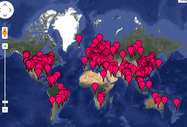
Ugh. We can do better. Much better. Unless our goal is to generate a ZOMGOSH THE WORLD IS PWND! response from our audience.

Mapping in D3

If you can’t tell, we really like the D3 framework for data visualization projects, and D3 excels at map making. So, we’re going to move our cartographic machinations from Google Maps to D3 and weave in some of the projection, scale and symbol concepts along the way. If you want to take a look at the source or just see the maps in a separate window, follow this link to a standalone version of the visualization.

Without further blathering on, here are the maps we’ll be referring to (you can take some time to explore the controls we’ve provided before the rest of the post).

Projections

The first difference you should notice (from the GMap) is that the earth looks skewed. That’s because we’ve defaulted to the Winkel Tripel projection and most folks are used to seeing the Mercator projection when they are looking at a 2D map. We’ve included Mercator as a menu selection as well as the equirectangular projection. Projections are nothing more than a mathematical mapping of 3D space onto a 2D plane. Each one skews reality in some way. Until we all start using holographic displays, we’re stuck with this mapping, so it’s up to us as communicators to use the right projection for the right purpose.

The Mercator projection is awesome for navigation but it’s terrible for communicating sizes (compare Greenland on a 3D globe to what you find on a Mercator map to see just how egregious the distortion is). Google defaults to Mercator (it is mainly for driving directions) but does have support for other projections, though most users never see anything but the default even when sites use the custom APIs for GMaps. In our sample maps visualization, you can switch between the projections to see the distortion on a macro level and on a regional level. In some projections, the points become mashed together and in others they spread apart even when zoomed in.

If you’re going to use a map, you need to consider the impact distortion has and ensure you’re not misrepresenting the data. Winkel Tripel is a good general purpose projection to standardize on since it tries to minimize the area, direction and distance distortions (that’s the ‘triple’ in Winkel Tripel). NASA uses the equirectangular projection quite a bit as do most organiations that create thematic maps and it isn’t a bad alternative to Winkel Tripel. However, as you can see in the example, you’ll need to use a bit more space in your layout.

NOTE: D3 makes many projections available and you should be able to slipstream additional ones into our base example to see the differences between all of them.

Scale

Scale is also important since we don’t have screens or printed materials the size of the planet and need to shrink down geographical elements to a manageble size. We won’t focus too much on scale since information security use cases for maps tend to not go down to street-level detail. We don’t usually display roads or other, similar features so we never really have to think about which elements to include or eliminate. In the example above, consider if it would have been helpful to include additional regional boundary details on the zoomed-in map of Europe or if we should have tossed in US county boundaries on the main overview map. Google (and your car’s GPS for that matter) makes many of these decisions for you so you may take them for granted.

You’ll need to assess whether detail should be added, removed or consolidated as you present your view(s) of reality to the consumers of your visualiztaion. We’ve stuck with country boundaries in both views in this example and consider that a a pretty safe default. If you’re just focusing (e.g. zooming-in) on certain countries or regions and are going to do more sub-region analyses (perhaps a US county-level choropleth) you’ll need to judiciously add more definition as the scale changes.

Also take note that most projections distort distance in the middle or at the edges, so be wary of using “equals” when stating scale since it’s unlikely you’ll be using a projection that affords this type of precision. Either using a pure ratio (i.e. “1:9,600“) or a sentence (e.g. “One inch represents 800 feet“) is suggested, with a graphical “stick” legend being your last choice (or a used as a secondary labeling element).

Symbols

While we let you play with projections, symbolic representation is the main focus of the example we’ve provided. Symbols tell us where “stuff” is and also, perhaps, “what” stuff is on a map. Hopefully you’ve fiddled with the controls in the above visualization to see how differences in opacity (how solid the fill of shape is) and size can impact what is being communicated. The Google map (which is similar to the ZeroAccess map created by F-Secure) shows points on a map with symbols. The default is a push-pin, but you can use almost any symbol you like. Again, this is great for directions but we’ll almost let the differences between the GMaps & D3 visualizations explain themselves.

Chaging opacity (I did say almost) will help convey (or distort) true density on a given place on a map. In this example, if we had let all the duplicate points on, the layered opacity values would continue to darken individual points. Varying point size can help communicate lack of precision or could be used if you’re going to size points proportionally. In this case, we created unique points from the original data since we just wanted to see how geographically diverse the “fly” nodes were. Giant symbols and even larger circles (or other symbol types) can make the spread of nodes seem much worse than they really are. This is especially true on the global map (go nuts with both sliders to pwn the whole world!). Ultimately, points on a map—especially/even infected system nodes—tend to track to population (this map is from the BBC):

However, we’ll be covering that topic a future post.

Wrapping Up Part 1

For now, realize that you as a map maker wield great power when you choose to use maps to convey meaning/information. Your audience is innately conditioned to accept what they see at face value and will react accordingly. When you’re displaying bots/nodes in a geospatial way choose your map asthetics wisely and with integrity. Unless you’re deliberately trying to mislead your consumers (or yourself) thoughtfully consider color, opacity, size, scale & projection to ensure your message is honest and definitely share the data you used to generate it so others can reproduce your results and, perhaps, challenge your assumptions.

Avoid defaulting to Google Maps and experiment with D3 (feel free to use our source as a starting point). If you feel “stuck” with Google Maps, take a look at their API to see how to modify the base theme to make your views more accurate and appealing to your audience.

We’ll leave you (until Part 2) with these two mapping gems from XKCD and a reminder to check out Chapter 5 of Data Driven Security : The Book for a more detailed look into telling data stories with maps.